SUM

Excel formulas are difficult tasks for users of this software. Learning Excel formulas is very important to help use Excel more effectively. In the previous lesson, I discussed the methods of entering a formula. In this lesson, I am going to teach you basic formulas.

SUM

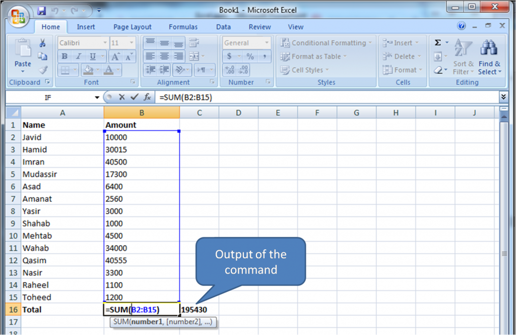
The SUM function is the most basic formula in Microsoft Excel. Using this formula, we can find the sum of two or more values in the cells. All formulas in Excel start with the equals sign “=” followed by a specific text formula. The SUM function is the must-know formula in Excel.

To perform this formula, enter the values to add together using the format =SUM(number1, [number2], …). The values, we need to enter into the formula can either be actual numbers or equal to the number in a specific cell of the spreadsheet. The example usage of this formula is:

=SUM(A2: H2) –Selection that sums the values of a row from A2 to AH.

=SUM(A2: A15) – Selection that sums the values of a column from A2 to A15.

=SUM(A2: A5, A9: A15, A20) – A complicated collection that sums values from range A2 to A5, skip A6, A7 and A8, adds A9 to A15, and then jumps to A20.

=SUM(A2: A10)/5 – Shows you can also turn your function into a formula.

Subtraction

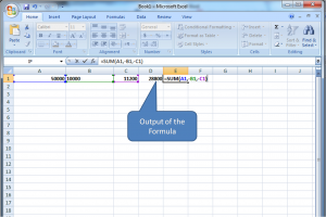
We can subtract multiple values from one another using the SUM formula, for example, “=SUM(A1, -B1, -C1)” with a negative sign before the cell whose value we need to subtract. The Figure below illustrates the output of the formula.

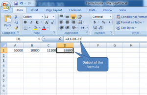
We can also use the format “=A1-B1” for subtraction. To subtract multiple values from one another we can just enter the formula “=A1-B1-C1”, the figure below illustrates the output of this command.

AVERAGE

The AVERAGE formula simply calculates the averages of data, such as the average number of shareholders in a given shareholding. To perform the average formula in Excel, enter the values, cells, or range of the cells you need to calculate the average.

The format of the formula is “=AVERAGE (number1, number2, etc.) or =AVERAGE (Start Value: End Value) for example “=Average(B2: B15). This formula will calculate the average of all the values or range of cells included in the B2 to B15 cells range. The figure below illustrates the average command.

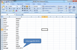
We can find the average using the formula =SUM(B2: B15)/14). B2 to B14, these are a total of 14 cells. The formula will divide the total B2 by B14 by the number 14.