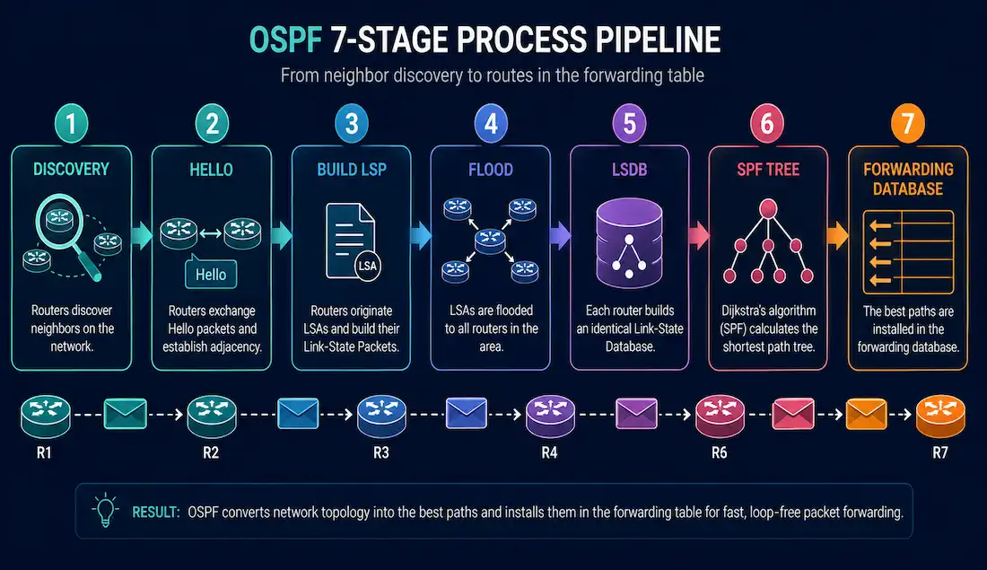
Link-state routing protocols are also known as shortest-path-first protocols. Every router running one maintains a complete picture of the entire network topology, built by having each router originate information about itself, its directly connected links, and the state of those links — then flooding that information to every other router in the area. OSPF is the most common real-world example, alongside IS-IS, and both rely on Dijkstra’s Shortest Path First (SPF) algorithm to calculate the actual best path once that shared topology picture is complete.
This guide walks through the entire link-state process end to end, using a concrete reference topology throughout, and ties together the OSPF-specific mechanics — LSA types, timers, cost calculation — that make the abstract process concrete in practice.
Example Topology
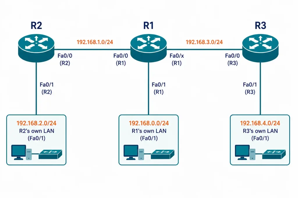
The examples throughout this guide reference a small three-router network:
| Router | Interface | Connects To | Network |
|---|---|---|---|
| R1 | Fa0/0 | R2 | 192.168.1.0/24 |
| R1 | Fa0/1 | Local LAN | 192.168.0.0/24 |
| R1 | (second interface) | R3 | 192.168.3.0/24 |
| R2 | Fa0/1 | Local LAN | 192.168.2.0/24 |
| R2 | Fa0/0 | R1 | 192.168.1.0/24 |
| R3 | Fa0/1 | Local LAN | 192.168.4.0/24 |
| R3 | Fa0/0 | R1 | 192.168.3.0/24 |
R1 sits at the center of this topology, connected to R2 on one side and R3 on the other, with its own directly attached LAN as well.
The Link-State Process, Step by Step
The process below applies identically to OSPFv2 (IPv4) and OSPFv3 (IPv6), differing mainly in addressing.
Step 1: Link and Link-State Discovery
Each router first learns about its own links. Once an interface is configured with an IP address and subnet mask and set to no shutdown, it becomes part of that network — physical connectivity alone isn’t enough until both configuration steps are complete. Once active, that directly connected network becomes an entry in the routing table automatically, even before any routing protocol starts exchanging information.
Link-state routers pass information about themselves, their directly connected links, and the state of those links to every other router in the area, unchanged. Every router ends up with identical raw information and independently calculates its own best paths from it.
R1’s link-state information, based on the reference topology:
| Link | Network | Interface | Neighbor | Type |
|---|---|---|---|---|
| Link 1 | 192.168.1.0/24 | Fa0/0 | R2 | Ethernet |
| Link 2 | 192.168.0.0/24 | Fa0/1 | (LAN, no router neighbor) | Ethernet |
| Link 3 | 192.168.3.0/24 | (second interface) | R3 | Ethernet |
Each link’s generated information includes the interface’s IP address and mask, the network type, the link’s cost, and any neighbor discovered on it.
Step 2: The Hello Protocol
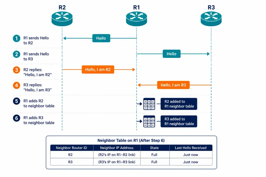
Routers use a Hello protocol to establish and maintain neighbor relationships on directly connected networks. A neighbor is simply another router running the same link-state protocol. Hello packets serve two purposes: initial neighbor discovery, and ongoing keep-alive monitoring.
R1 sends Hello packets out every active interface. R2 and R3 respond with their own Hello packets, identifying themselves (“Hello, I am R2” / “Hello, I am R3”), which lets R1 add each one to its neighbor table by actual router identity, not just by interface. If an interface has no responding neighbor — R1’s LAN-facing Fa0/1, for instance — the process simply doesn’t continue on that interface. That’s not an error; it’s just an interface with no protocol neighbor to adjacent with.
Hello packets continue as an ongoing keep-alive after the initial exchange. If Hello packets stop arriving from a specific neighbor, that neighbor is eventually marked unreachable and removed from the adjacency table.
OSPF Hello timing specifics: Hello packets themselves are never stored in the link-state database — they exist purely for discovery and liveness detection. On broadcast networks, if no Hello has been received from a neighbor for 40 seconds (the default Dead Interval, four times the default 10-second Hello Interval), that neighbor is marked down.
Brief outages are handled gracefully — a link that drops and recovers within roughly 20 seconds may not register as a meaningful disruption at all. For longer outages, LSA aging takes over: every LSA carries a maximum age of 3600 seconds (1 hour), per RFC 2328, after which it’s flushed from the database if not refreshed and must be reflooded as new information once the link returns — effectively looking like a brand-new route to the rest of the network rather than a restored one.
Step 3: Building the Link-State Packet (LSP / LSA)
Once adjacencies are established, each router builds a Link-State Packet — called an LSA specifically in OSPF terminology — containing the state of each directly connected link: neighbor identity, link type, and cost.
R1’s LSP, based on the reference topology:
- R1 → R2; Fa0/0; network 192.168.1.0/24; Cost 1
- R1 → local LAN; Fa0/1; network 192.168.0.0/24; Cost 1
- R1 → R3; second interface; network 192.168.3.0/24; Cost 1
LSPs aren’t sent periodically the way Hello packets are. They’re sent once during initial protocol startup, and afterward only when a genuine topology change occurs — a link failing, recovering, or a new network being added.
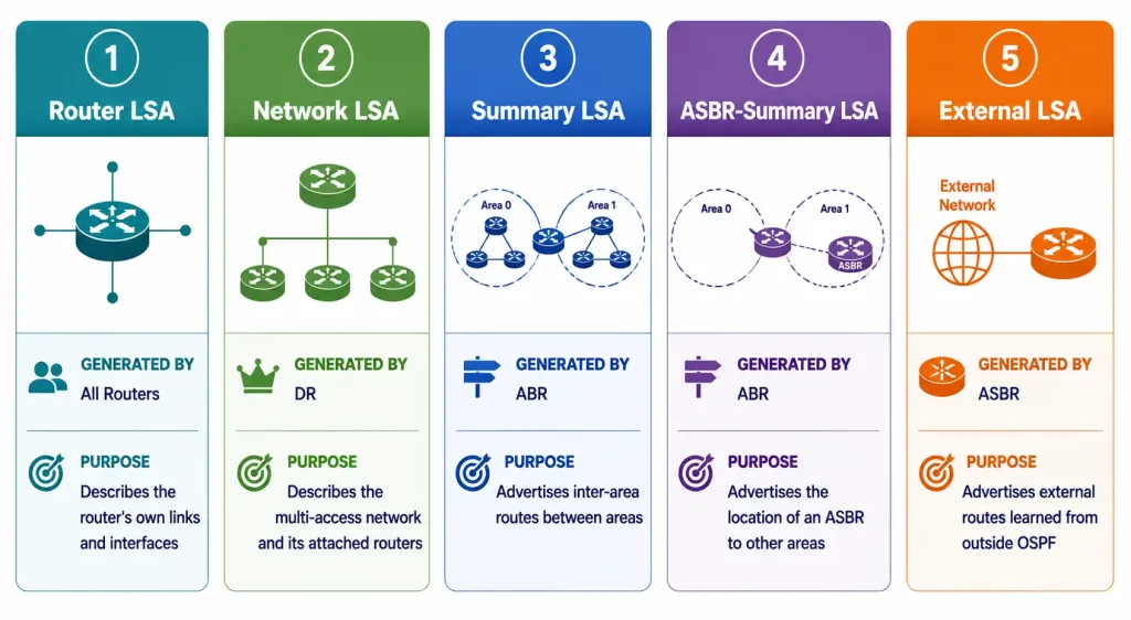
OSPF specifically classifies LSAs into five types, each generated by a different router role:
| LSA Type | Name | Generated By | Purpose |
|---|---|---|---|
| Type 1 | Router LSA | Every OSPF router | Describes the router’s own links and their costs |
| Type 2 | Network LSA | The DR on a multi-access segment | Describes the segment and its attached routers |
| Type 3 | Summary LSA | Area Border Routers (ABRs) | Advertises inter-area routes into another area |
| Type 4 | ASBR Summary LSA | ABRs | Advertises the location of an ASBR to other areas |
| Type 5 | External LSA | AS Boundary Routers (ASBRs) | Advertises routes learned from outside the OSPF domain |
Step 4: Flooding the LSP
After building its LSP, each router floods it to all of its neighbors. Neighboring routers store it in their own link-state database and reflood it out every interface except the one it arrived on. This repeats hop by hop until every router in the area has a copy.
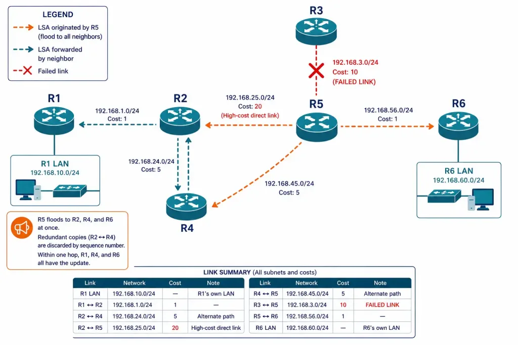
To see why flooding matters more as a network grows, consider a separate, larger illustrative topology — six routers rather than three, introduced here specifically to show flooding at scale rather than as an extension of the R1/R2/R3 reference network above. (This example reuses the labels R1, R2, and R3 for convenience, but they represent different routers, with different subnets, than the reference topology used elsewhere in this guide.) R1 (with its own LAN) connects to R2, which connects onward to R5 through two possible paths — a direct link (cost 20) and an alternate path via R4. R5 also connects directly to R3 and out to R6 (with its own LAN).
If the link between R3 and R5 goes down, R5 generates an updated LSP and floods it out every surviving interface at once — to R2, R4, and R6 simultaneously, not sequentially through any one of them. R2 and R4 each reflood the update toward each other, arriving redundantly on both sides since each already received it directly from R5; every router recognizes and discards that redundant copy by its sequence number rather than reflooding it further. Within a few seconds, every router in the topology — including R1 and R6 at opposite ends of the network — has the update, with no need for a separate individual notification to each router.
Each LSP carries a sequence number and aging information, letting every router distinguish genuinely new information from a stale duplicate already in its database — once a router has processed a given LSP’s current sequence number, it discards redundant copies rather than reflooding them again, which is exactly what keeps the flooding process from looping indefinitely. Because flooding completes before SPF calculation begins, and propagates hop by hop rather than waiting on any periodic timer, link-state protocols generally achieve much faster convergence than distance-vector protocols.
Step 5: Building the Link-State Database
Every router stores the LSPs it receives from every other router in the area, forming a complete map of that area’s topology — also called the topological database. Every router within the same area maintains an identical copy, built from router LSAs, network LSAs, and, in non-stub areas, summary and external route advertisements. Verify it directly with show ip ospf database.
Each router maintains a separate link-state database per area it belongs to, since both flooding and SPF calculation happen independently within each area. This is exactly why link-state databases must be identical across every router in the same area: any inconsistency would cause different routers to calculate different, potentially conflicting paths to the same destination. For CCNP-level scalability, inter-area routing relies on Type 3 summary LSAs from ABRs rather than flooding full topology detail across area boundaries.
Step 6: Running the SPF Algorithm
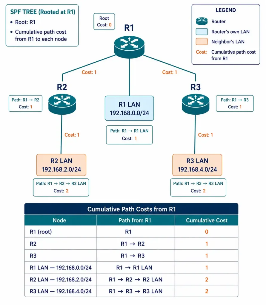
Once a router has received LSPs from every other router in its area, it uses its complete link-state database and the SPF (Dijkstra) algorithm to independently build its own shortest-path tree — starting from its own directly connected networks and costs, then working outward through the received LSPs to calculate the lowest cumulative-cost path to every known network.
Using the reference topology, R1’s SPF tree roots at R1, with direct branches to R2 (cost 1), R3 (cost 1), and its own local LAN (cost 1) as a leaf off the root. Every router in the area builds this same tree independently, from the identical shared database.
A slightly more complex example shows why total cost matters more than hop count: in a triangle topology where the A–B link costs 1, the B–C link costs 1, and the direct A–C link costs 10, router A’s SPF tree prefers path A–B–C (total cost 2) over the direct A–C link (cost 10), even though A–B–C takes an extra hop.
SPF calculation is genuinely CPU-intensive, which is why large networks benefit from partial (incremental) SPF — recalculating only the affected branch for a minor change rather than rebuilding the entire tree. Costs themselves are based on interface bandwidth, using the formula reference bandwidth ÷ interface bandwidth. Cisco’s default reference bandwidth is 100 Mbps, which is worth knowing has become outdated on modern high-speed links — without manually raising it with auto-cost reference-bandwidth, every interface faster than 100 Mbps calculates to the same minimum cost of 1, making OSPF effectively blind to the real difference between, say, a 1 Gbps and a 10 Gbps link.
Step 7: Populating the Forwarding Database
The SPF tree’s lowest-cost paths populate the router’s actual routing table, inspected with the familiar show ip route. From here, packet forwarding follows the standard longest-prefix-match logic covered in the routing table lookup guide — SPF-derived routes are simply another source competing within that same overall process. Where multiple equal-cost paths exist, OSPF supports load balancing across up to 4 paths by default on Cisco IOS, configurable up to 16.
DR and BDR Election on Multi-Access Networks
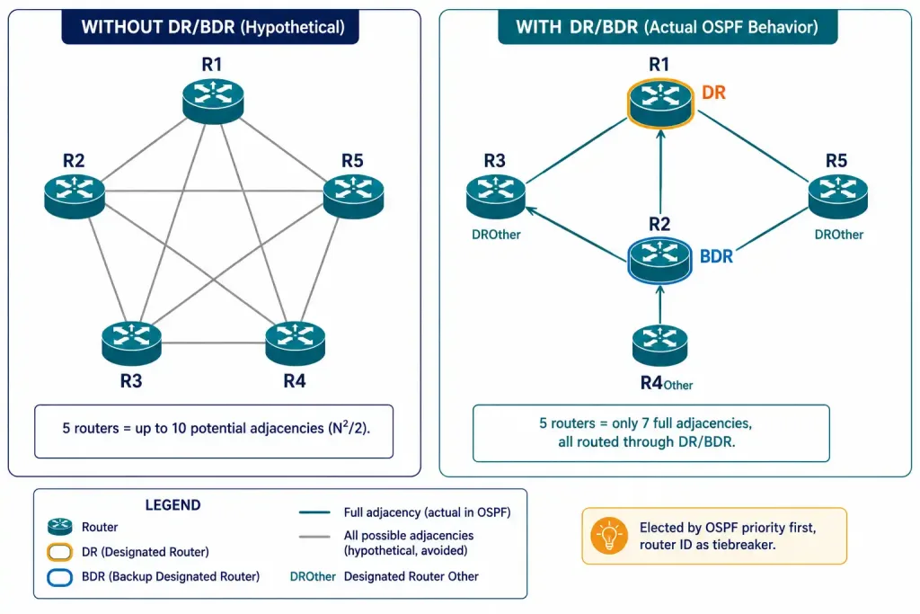
On a multi-access segment like Ethernet with several OSPF routers, forming a full adjacency between every pair of routers would create unnecessary redundant LSA exchange — with N routers on a segment, that’s roughly N²/2 potential adjacencies. Instead, OSPF elects a Designated Router and a Backup Designated Router, based on OSPF priority first and router ID as the tiebreaker; every other router forms a full adjacency only with the DR and BDR, dramatically reducing the flooding overhead needed to keep the segment synchronized.
Summary of the Link-State Process
- Each router learns about its own directly connected networks and links by detecting interfaces in the up state.
- Routers exchange Hello packets with neighbors on directly connected networks, forming adjacencies.
- Each router builds a Link-State Packet (LSA in OSPF) describing each directly connected link, neighbor, link type, and cost.
- Each router floods its LSP to all neighbors, who store and reflood it onward until every router in the area has a copy.
- Every router uses its now-complete link-state database to independently build an SPF tree via Dijkstra’s algorithm, calculating the best path to every destination.
- Best paths populate the forwarding database — the actual routing table used for packet forwarding.
Important Terms
| Term | Definition |
|---|---|
| Topological database | The complete set of information collected from LSAs/LSPs for an area |
| SPF algorithm | The Dijkstra-based algorithm used to calculate the shortest-path tree from the link-state database |
| Routing table | The final list of known destination networks and the interface/next-hop used to reach each |
| LSA | Link-State Advertisement — the OSPF-specific term for the packet of routing information exchanged between routers |
| LSP | Link-State Packet — the general term, used across link-state protocols, for the same underlying concept |
Advantages and Disadvantages
Advantages
- Fast convergence — LSPs flood immediately on receipt, without waiting on any periodic timer.
- Full topological map — every router builds a complete SPF tree of the area, calculating genuinely shortest paths rather than relying on secondhand hop-count information.
- Hierarchical design — multiple areas allow route summarization and far better scalability than a single flat topology.
- Event-driven updates — after initial flooding, LSPs are sent only when something actually changes, and carry only the affected information.
Disadvantages
- Memory requirements — maintaining a full link-state database and SPF tree needs meaningfully more memory than a distance-vector protocol’s simpler table.
- Processing requirements — the Dijkstra algorithm demands more CPU than simpler algorithms like Bellman-Ford, since it computes a complete shortest-path tree rather than incrementally comparing distances.
- Bandwidth requirements — initial LSP flooding, and reflooding after major topology changes, consumes real bandwidth, particularly noticeable in unstable networks with frequent link flaps.
Protocols That Use Link-State Routing
OSPF is the most widely deployed link-state protocol, originally designed by the IETF starting around 1987. OSPFv2, for IPv4, is defined in RFC 2328. OSPFv3, for IPv6 (and also capable of supporting IPv4 address families), was originally defined in RFC 2740 and has since been superseded by RFC 5340, the current standard. OSPF is an open standard supported on virtually every enterprise routing platform, uses Dijkstra’s algorithm for loop-free topology, and is classless, supporting VLSM and hierarchical area-based summarization.
IS-IS is an open standard designed by the International Organization for Standardization, described in ISO 10589. It was originally built for the OSI protocol suite rather than TCP/IP; Integrated (or Dual) IS-IS later added IP support alongside OSI. IS-IS is particularly associated with internet service providers and carriers, valued for scaling to very large networks — often considered easier to scale than OSPF at the largest sizes — and carries reachability data that’s largely agnostic to what that payload actually contains.
Link-State vs. Distance-Vector, at a Glance
| Aspect | Link-State (OSPF / IS-IS) | Distance-Vector (RIP) |
|---|---|---|
| Topology view | Full map via LSDB | Partial, learned secondhand from neighbors |
| Updates | Event-triggered, partial | Periodic, full table |
| Convergence | Fast — typically seconds | Slow — can take minutes |
| Loop prevention | SPF algorithm | Split horizon, route poisoning |
| Scalability | High, with areas | Low — limited by hop count |
| Resource use | Higher CPU and memory | Lower CPU, more bandwidth-heavy over time |
CCNA and CCNP Exam Pointers
- Link-state protocols: OSPF and IS-IS, both using the Dijkstra (SPF) algorithm.
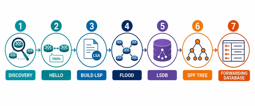
- Process order: Discovery → Hello → Build LSP → Flood LSP → Build LSDB → Run SPF → Populate Forwarding Database.
- OSPF default timers: Hello 10s / Dead 40s on broadcast networks.
- LSA MaxAge = 3600 seconds (1 hour) — after this, an LSA is flushed and must be reflooded as new.
- LSPs/LSAs are not periodic after initial flooding — sent only on a genuine topology change.
- Link-state databases must be identical across all routers in the same area for consistent SPF calculation.
- OSPFv2 = RFC 2328 (IPv4); OSPFv3 = RFC 5340 (current, supersedes RFC 2740), IPv6, also supports IPv4 AF.
- IS-IS: ISO 10589, originally OSI-only; Integrated/Dual IS-IS adds IP support.
Frequently Asked Questions
What are link-state routing protocols, and how do they differ from distance-vector protocols?
Link-state routing protocols, also called shortest-path-first protocols, maintain a complete view of the network topology by having every router flood information about itself and its directly connected links to every other router in the area. Each router then independently calculates the shortest path to every destination using the SPF (Dijkstra) algorithm, based on that identical shared topology data. This differs fundamentally from distance-vector protocols like RIP, which only know what their immediate neighbors report secondhand, with no independent view of the broader topology.
How does the discovery and Hello process work?
A router first learns about its own directly connected networks once an interface is configured with an IP address and set to no shutdown — this automatically creates a routing table entry before any protocol exchange begins. From there, the Hello protocol establishes neighbor relationships on directly connected networks, with routers identifying themselves to each other and continuing to exchange Hellos afterward purely as a keep-alive function. If Hello packets stop arriving from a neighbor for the Dead Interval — 40 seconds by default on OSPF broadcast networks — that neighbor is marked unreachable and removed from the adjacency table.
What is an LSP or LSA, and what information does it contain?
A Link-State Packet (called an LSA specifically in OSPF) contains the state of each of a router’s directly connected links — the interface’s address and mask, the network type, the link’s cost, and any neighbor discovered on it. This information is flooded, unchanged, to every other router in the area, forming the raw material each router uses to build its own link-state database. OSPF additionally classifies LSAs into five distinct types, each generated by a different router role, depending on what kind of information they’re advertising and where in the topology they originate.
How does LSP flooding work, and why doesn’t it loop forever?
After building its LSP, a router sends it to all its neighbors; each receiving router stores it and reforwards it out every interface except the one it arrived on, continuing hop by hop until every router in the area has a copy. Sequence numbers and aging information included in each LSP let routers recognize and discard duplicate or stale copies, which is exactly what prevents the flooding process from looping indefinitely rather than eventually settling once every router is synchronized.
How does the SPF algorithm build the routing table, and why might a longer path win?
Each router runs Dijkstra’s algorithm against its own link-state database, treating itself as the root, to calculate the lowest cumulative-cost path to every other destination in the topology — and because this is based on total cost rather than hop count, a path with more hops can still win if its combined cost is genuinely lower than a shorter, more expensive alternative. Because every router in an area shares an identical link-state database, each router’s independently calculated SPF tree stays consistent with every other router’s, which is essential for loop-free, accurate routing across the entire area.
What are OSPF and IS-IS, and how do they compare?
OSPF and IS-IS are the two standard link-state routing protocols, both built on Dijkstra’s SPF algorithm but developed under different standards bodies — OSPF by the IETF (RFC 2328 for IPv4, RFC 5340 for IPv6), and IS-IS by the ISO (ISO 10589), originally for the OSI protocol suite before Integrated IS-IS added IP support. OSPF is the more common choice in enterprise networks and is supported on virtually every routing platform, while IS-IS is particularly associated with internet service providers and large carrier networks, often considered to scale more easily at the very largest network sizes.