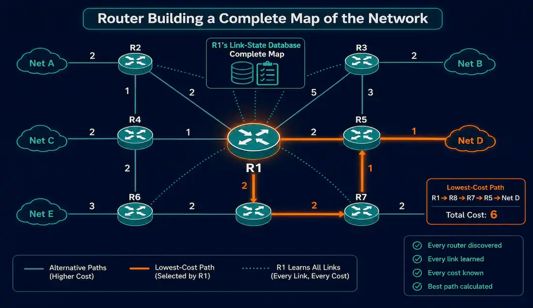
Efficient routing matters most in complex topologies with many possible paths between two points. The Shortest Path First protocol — better known as link-state routing — uses Edsger Dijkstra’s shortest-path algorithm to work out the genuinely optimal path for forwarding packets, rather than relying on a simpler metric like hop count. Open Shortest Path First and IS-IS (Intermediate System-to-Intermediate System) are the two protocols that put this algorithm to work in real networks. Both are meaningfully more complex than distance-vector protocols like RIP, but in exchange offer faster convergence and far better scalability for enterprise-scale networks.
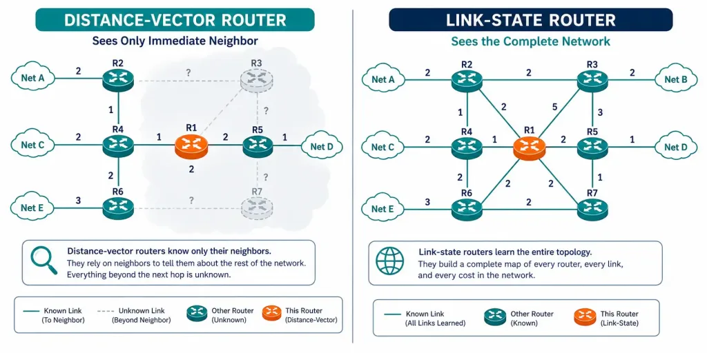
[See Infographic: Link-State vs Distance-Vector at a Glance]
Link-State vs. Distance-Vector, Side by Side
| Feature | Link-State (OSPF / IS-IS) | Distance-Vector (RIP) |
|---|---|---|
| Algorithm | Dijkstra’s SPF | Bellman-Ford |
| Convergence | Fast — event-driven | Slow — periodic updates |
| Scalability | High — hierarchical design | Low — flat topology |
| CPU/memory usage | Higher | Lower |
| Metric | Cost, based on bandwidth | Hop count |
The core philosophical difference: a distance-vector protocol like RIP only knows what its immediate neighbors tell it, one hop at a time. A link-state protocol builds a complete map of the entire topology — every router, every link, every cost — and calculates the best path itself using that full picture, rather than trusting secondhand information passed router to router.
Dijkstra’s Algorithm
Dijkstra’s algorithm was published in 1959 by computer scientist Edsger Dijkstra, and it’s the algorithm both OSPF and IS-IS use to calculate the best path from a source to every other destination in the network. It’s commonly called the shortest path first algorithm for exactly this reason. The algorithm works by summing the costs along every possible path from source to destination, and selecting whichever path has the lowest total cost as the best route.
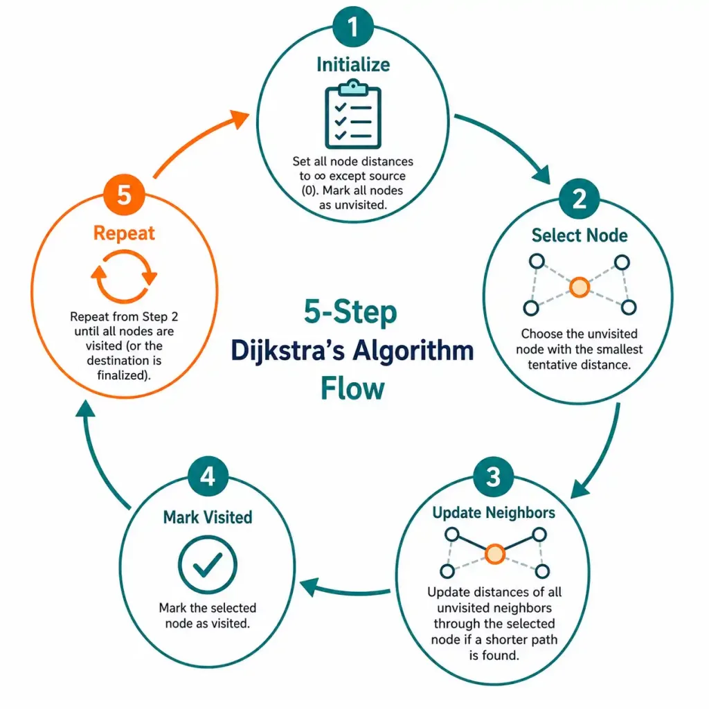
The algorithm proceeds in five steps:
- Initialize. Set the distance to the source router as 0, and to every other router as infinity. Create a set containing every unvisited router in the topology.
- Select a node. Choose the unvisited router with the smallest known distance from the source.
- Update neighbors. For the selected router, calculate the distance to each of its directly connected neighbors. If a shorter path to any neighbor is found through this router, update that neighbor’s recorded distance.
- Mark visited. Mark the selected router as visited, and remove it from the unvisited set.
- Repeat. Continue selecting, updating, and marking until every router has been visited or no further updates are possible.
The end result is a shortest-path tree rooted at the source router, giving the lowest-cost path to every other router in the topology — not just to one specific destination.
[See Infographic: The Five Steps of Dijkstra’s Algorithm]
Illustrative Scenario: Why Fewest Hops Isn’t Always Cheapest
The following is an illustrative scenario built to demonstrate the concept clearly, with costs I’ve calculated and verified myself, rather than a claim about any specific real-world topology.
Consider a small network with routers R1 through R6, where R1’s LAN needs to reach R6’s LAN. Suppose there are three possible paths, each with a link cost assigned to every hop:
- Path A (R1–R2–R3–R6): link costs 5, 20, 25 → total cost 50
- Path B (R1–R2–R5–R6): link costs 5, 20, 15 → total cost 40, and only 3 hops — the fewest of any path
- Path C (R1–R2–R4–R5–R6): link costs 5, 8, 6, 15 → total cost 34, but 4 hops — one more hop than Path B
Even though Path B has the fewest hops, Path C has the lowest total cost, because the R2–R4–R5 segment (cost 8 + 6 = 14) is cheaper overall than the direct R2–R5 segment (cost 20), despite adding an extra hop. Dijkstra’s algorithm — and therefore OSPF and IS-IS — selects Path C, the genuinely cheapest path, rather than Path B, the path with fewer hops. This is exactly the distinction that separates link-state routing from a hop-count-based protocol like RIP: RIP would have selected Path B purely because it has fewer hops, with no way to account for the fact that Path C is actually less costly overall.
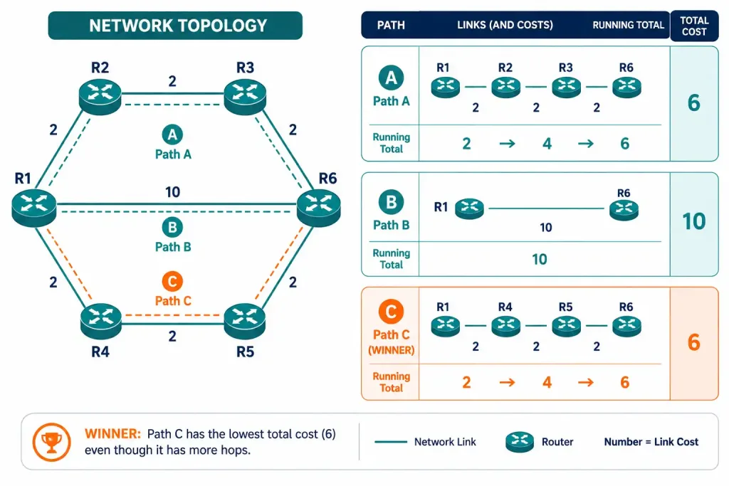
[See Infographic: Fewest Hops vs Lowest Cost — Same Topology, Different Winners]
Pros and Cons of Link-State Protocols
Pros:
- Fast convergence. Event-triggered updates mean topology changes propagate quickly, minimizing downtime after a link failure.
- Loop-free routing. Full topology awareness, maintained through each router’s link-state database (LSDB), prevents the routing loops that can affect distance-vector protocols.
- Scalability. Hierarchical design — areas in OSPF, levels in IS-IS — lets link-state protocols scale to large enterprise networks in a way flat distance-vector designs can’t.
- VLSM and CIDR support. Link-state protocols advertise subnet masks natively, making them a natural fit for efficient, classless IP addressing.
Cons:
- Higher resource usage. Maintaining a full link-state database and running SPF calculations demands more CPU and memory than a simple distance-vector protocol.
- Greater complexity. Configuration and troubleshooting are more involved than RIP, with more moving parts to understand — areas, LSA types, adjacency states.
- Flooding overhead. Link-state advertisements can consume meaningful bandwidth if not tuned appropriately, particularly on networks with frequent topology changes.
OSPF mitigates much of this complexity through its area structure, limiting how far LSA flooding needs to travel. IS-IS is often the preferred choice in large service-provider networks specifically because of its protocol-independent design and flexibility at very large scale.
OSPF vs. IS-IS
Both uses Dijkstra’s SPF algorithm, but they differ in meaningful ways:
- OSPF is IPv4/IPv6-specific, structured around areas with a mandatory backbone (Area 0), and is the more common choice in enterprise networks.
- IS-IS is protocol-independent, originally designed around CLNS rather than IP directly, and structured around levels (L1 and L2) rather than OSPF’s area model. It’s frequently the preferred choice in very large-scale deployments, particularly ISP backbones.
A useful distinction for CCNP-level study: IS-IS doesn’t require a mandatory backbone area the way OSPF requires Area 0, which gives it more topological flexibility during network migrations and redesigns.
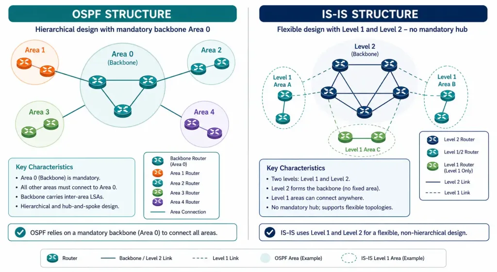
[See Infographic: OSPF’s Area Model vs IS-IS’s Level Model]
OSPF Packet Types and Convergence
It relies on five distinct packet types to build and maintain its link-state database:
- Hello — discovers neighboring routers and establishes adjacencies.
- Database Description (DBD) — summarizes the contents of a router’s link-state database.
- Link-State Request (LSR) — requests specific link-state advertisements a router is missing.
- Link-State Update (LSU) — floods link-state advertisements (LSAs) to neighbors.
- Link-State Acknowledgment (LSAck) — confirms receipt of an LSU.
Convergence happens once every router in the OSPF domain has synchronized link-state databases and independently run the SPF algorithm on that shared topology data. When a link fails, the affected router floods updated LSAs describing the change, and other routers — rather than recalculating their entire shortest-path tree from scratch — typically perform a partial SPF recalculation limited to the affected portion of the topology, which keeps convergence fast even in larger networks.
Verifying OSPF Configuration
A handful of commands cover most day-to-day OSPF verification needs:
Router# show ip ospf neighbor
Router# show ip ospf database
Router# show ip route ospf
show ip ospf neighbor confirms which adjacencies are actually up and in the expected state. show ip ospf database displays the router’s link-state database — useful for confirming every router in the area agrees on the topology. show ip route ospf filters the routing table down to just the routes OSPF has installed. For troubleshooting adjacency problems specifically, debug ip ospf adj shows the live adjacency formation process, though it should be used briefly and cautiously given the volume of output it generates.
Partial vs. Full SPF Recalculation
Running the full Dijkstra algorithm from scratch across an entire large topology is expensive — it’s exactly the kind of CPU overhead link-state protocols are criticized for. Modern OSPF and IS-IS implementations avoid doing this on every single topology change by distinguishing between two kinds of recalculation.
A full SPF run recalculates the shortest-path tree for the entire topology from the source router outward. This happens when something fundamental changes — a router joins or leaves the area, or the topology changes in a way that could affect paths broadly across the network.
A partial SPF run (sometimes called a partial route calculation, or PRC) only recalculates the affected portion of the topology — typically when a change affects reachability to a specific destination network without altering the router-to-router topology itself, such as a single stub network appearing or disappearing behind an otherwise unchanged router. Since the router-level topology hasn’t actually changed, there’s no need to rebuild the entire shortest-path tree; only the specific branch affected by the change needs to be recalculated.
This distinction is a large part of why link-state protocols manage to combine fast convergence with reasonable CPU usage even on larger networks: rather than treating every change as equally expensive, the protocol scales its response to match the actual scope of what changed. A single host route disappearing at the edge of a large OSPF area shouldn’t — and, with partial SPF, doesn’t — require every router in that area to recompute its entire shortest-path tree from zero.
Frequently Asked Questions
What is the SPF protocol?
It, more commonly called link-state routing, uses Dijkstra’s algorithm to calculate the genuinely lowest-cost path between routers, based on a complete map of the network topology rather than secondhand hop-count information. OSPF and IS-IS are the two protocols that implement this approach in practice, each building a full link-state database and independently calculating shortest paths from it. This gives link-state protocols faster convergence and far better scalability than distance-vector protocols like RIP, particularly in large or complex enterprise topologies.
How does Dijkstra’s algorithm work in OSPF?
The algorithm starts by setting the source router’s distance to 0 and every other router’s distance to infinity, then repeatedly selects the nearest unvisited router, updates the recorded distance to its neighbors if a shorter path is found through it, and marks that router visited. This process repeats until every router in the topology has been visited, producing a complete shortest-path tree rooted at the source router. OSPF runs this calculation independently on every router, using the shared link-state database every router in the area maintains, which is what guarantees loop-free routing throughout the domain.
What are the pros and cons of link-state protocols?
The main advantages are fast, event-driven convergence, strong scalability through hierarchical area or level design, and native support for VLSM and CIDR through explicit subnet mask advertisement. The main disadvantages are higher CPU and memory usage from maintaining a full link-state database and running SPF calculations, along with meaningfully greater configuration and troubleshooting complexity compared to a simple protocol like RIP. OSPF is generally the better fit for enterprise networks, while IS-IS is often preferred in very large service-provider environments due to its flexibility and protocol independence.
Why might a path with more hops actually be the best path?
Because link-state routing selects the path with the lowest total cost, not the path with the fewest hops — and those aren’t always the same path. If one segment of a shorter path carries an unusually high cost, perhaps due to a slow or congested link, a longer path made up of several cheaper links can end up with a lower total cost overall. This is exactly the distinction that separates link-state protocols like OSPF from hop-count-based protocols like RIP, which would select the fewest-hop path regardless of the actual cost or bandwidth involved.
How do you verify OSPF configuration on a router?
Use show ip ospf neighbor to confirm adjacencies have formed correctly, show ip ospf database to inspect the router’s link-state database, and show ip route ospf to see exactly which routes OSPF has installed in the routing table. For troubleshooting adjacency problems specifically, debug ip ospf adj shows the live formation process step by step, which is useful for diagnosing why two routers aren’t becoming neighbors as expected — though it should be used sparingly given how much output it can generate on a busy router.