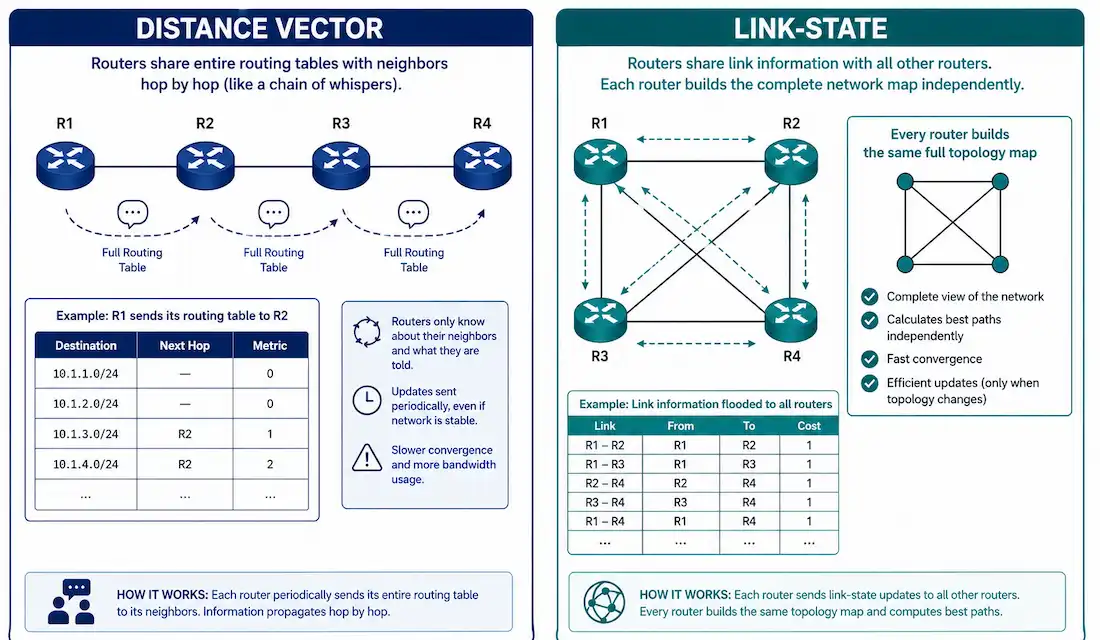
Every dynamic routing protocol has to solve the same underlying problem: how does a router, knowing only about its own directly connected networks, learn about everything else and figure out the best path to reach it? The answer comes down to one of two fundamentally different approaches — distance vector or link-state — and understanding the real difference between them is what makes RIP, EIGRP, and OSPF’s behavior actually make sense, rather than just being three protocols to memorize separately.
This guide covers both algorithm types in depth, why distance-vector protocols are prone to routing loops and how split-horizon fixes it, full worked configuration for RIP, OSPF, and EIGRP, and real troubleshooting steps for each.
What Dynamic Routing Actually Does
Dynamic routing protocols automate what static routing requires by hand: network discovery, maintaining accurate routing tables, and automatically selecting the best path as the network changes. Unlike a static route, a dynamically learned route updates itself when a link fails or a new network appears, without any administrator intervention.
The major dynamic routing protocols split by IP version:
- EIGRP and EIGRP for IPv6 — Enhanced Interior Gateway Routing Protocol
- OSPF (IPv4) and OSPFv3 (IPv6) — Open Shortest Path First
- IS-IS — Intermediate System-to-Intermediate System
- RIP and RIPng — Routing Information Protocol (and its IPv6 successor)
All of these rely on one of two underlying routing algorithms: distance vector or link-state. EIGRP is often described as a hybrid of the two, though current Cisco terminology more precisely calls it an “advanced distance-vector” protocol, since its core DUAL algorithm is fundamentally distance-vector in nature even with link-state-like enhancements layered on top.
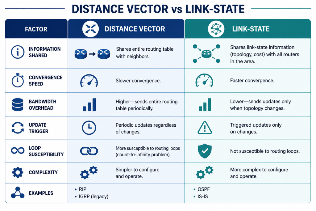
[See Infographic: Distance Vector vs Link-State Algorithm Comparison]
Distance Vector Routing Algorithms
Distance-vector protocols work on a simple principle, often called “routing by rumor”: each router tells its directly connected neighbors what it knows, and trusts what its neighbors tell it in return, without independently verifying the actual topology beyond its own directly connected links.
This is powered by the Bellman-Ford algorithm. Every router maintains a distance vector table listing the distance to every known destination and the direction (which neighbor) to reach it. Two values matter for each entry:
- Distance: typically hop count — the number of routers between here and the destination.
- Vector: the direction, meaning which neighboring router leads toward that destination.
RIP is the classic distance-vector protocol, using pure hop count as its metric, capped at a maximum of 15 hops — a 16th hop is treated as unreachable. This ceiling is a real, meaningful limitation: RIP simply can’t be used on any network where a valid path might legitimately require more than 15 hops.
Routers running a distance-vector protocol periodically advertise their entire routing table to directly connected neighbors, without waiting for a specific trigger. The receiving router doesn’t send an acknowledgment back — this keeps protocol overhead low, but it also means updates rely purely on periodic timing rather than confirmed delivery.
Why Distance Vector Protocols Are Prone to Routing Loops
Because each router only trusts what its neighbors report, without any independent view of the broader topology, a distance-vector protocol can be fooled by stale information. Consider three routers in a line: A–B–C. If the link from C to a destination network fails, but C hasn’t yet told B, and B still has an old route pointing through C, a routing loop can form — B might send traffic back toward C believing C still has a valid path, while C (having lost its own route) sends it right back to B.
Split horizon is the standard fix: a router never advertises a route back out the same interface it learned that route from. This single rule prevents an entire category of loops, since a router can’t hear its own advertised route echoed back to it as if it were new information from a neighbor. Other loop-prevention techniques — route poisoning, holddown timers, and triggered updates — layer additional protection on top of split horizon for more complex topology change scenarios.
Link-State Routing Algorithms
Link-state protocols take a fundamentally different approach: instead of trusting secondhand information from neighbors, every router builds its own complete, independent map of the entire network topology (within its area, for a protocol like OSPF), then calculates the best path itself.
Each router running a link-state protocol floods Link-State Advertisements (LSAs) — small packets describing its own directly connected links and their state — to every other router within the same area, using multicast rather than broadcasting to the entire network, which keeps overhead manageable even as the network grows.
Key terms:
- Link-State Advertisement (LSA): a packet describing a link’s status, flooded whenever that link’s state changes, not just on a periodic timer.
- Topological database (Link-State Database, LSDB): the complete set of LSAs a router has received, describing the entire area’s topology in detail.
- SPF algorithm: Dijkstra’s shortest path first algorithm, run independently by every router in the area against its own LSDB, computing the actual shortest-path tree to every destination.
- Routing table: the final list of best routes, built from the SPF tree’s results.
OSPF is the primary link-state protocol taught at the CCNA/CCNP level. Its hierarchical area structure — with Area Border Routers (ABRs) connecting multiple areas back to a backbone Area 0 — keeps flooding and SPF calculation overhead manageable even on large networks, since a router only needs a complete topology map of its own area, not the entire organization.
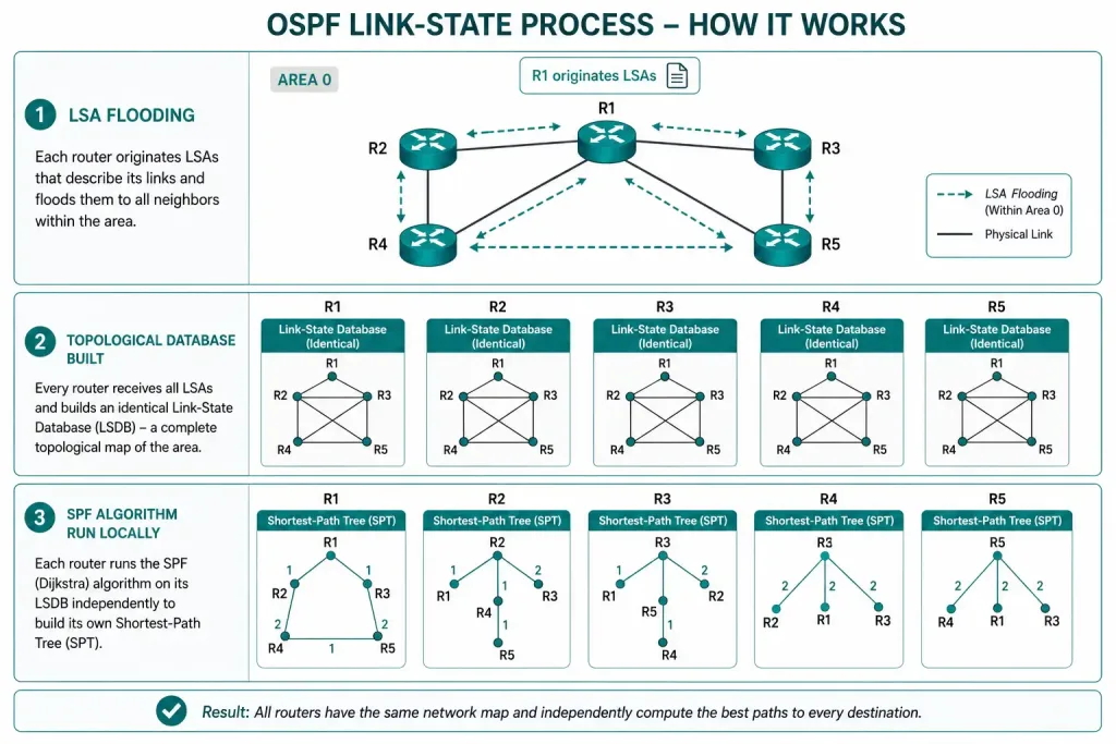
[See Infographic: How Link-State Flooding and SPF Calculation Work]
Distance Vector vs. Link-State: Direct Comparison
| Factor | Distance Vector | Link-State |
|---|---|---|
| Information shared | Entire routing table, periodically | Individual link status, on change |
| View of topology | Only through neighbors’ reports | Complete, independently calculated |
| Convergence speed | Slower | Faster |
| CPU/memory overhead | Lower | Higher (full topology database, SPF calculation) |
| Loop susceptibility | Higher (mitigated by split horizon and related techniques) | Lower (full topology awareness prevents most loop scenarios) |
| Example protocols | RIP | OSPF, IS-IS |
Convergence: Why the Algorithm Choice Matters in Practice
Convergence — how quickly every router in a network agrees on a consistent, correct view of the topology after a change — is where the distance-vector versus link-state distinction has the most real-world impact, beyond just exam trivia.
A distance-vector protocol’s convergence time is fundamentally limited by how quickly change information propagates hop by hop, router by router, each one waiting on its neighbor before it can update and pass the news along. RIP compounds this with its own periodic update timer (every 30 seconds by default), meaning a change can take a genuinely long time — potentially minutes — to fully propagate across a larger network, even with triggered updates helping to speed things along.
A link-state protocol converges faster specifically because every router calculates its own routes independently once it has the updated topology information, rather than waiting on a chain of hop-by-hop updates. OSPF’s flooding mechanism gets updated link-state information to every router in the area quickly, and each router’s own SPF calculation happens locally and in parallel with every other router’s calculation — there’s no sequential dependency chain the way there is with distance-vector’s hop-by-hop update propagation.
This is precisely why OSPF and EIGRP (with its own fast convergence via DUAL) are standard choices for larger, more dynamic networks, while RIP remains genuinely appropriate only for small, stable networks where slow convergence after a rare topology change is an acceptable trade-off for RIP’s configuration simplicity.
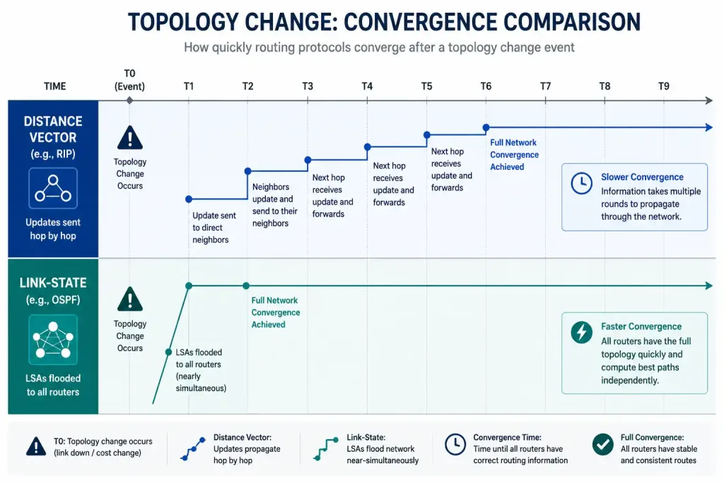
[See Infographic: Convergence Speed Comparison]
Configuring RIP, OSPF, and EIGRP
RIP:
Router(config)# router rip
Router(config-router)# version 2
Router(config-router)# network 192.168.1.0
version 2 enables RIPv2, which supports classless routing (VLSM) and multicast updates — RIPv1 is legacy and generally shouldn’t be used on any current network, since it lacks both of these.
OSPF:
Router(config)# router ospf 1
Router(config-router)# network 192.168.1.0 0.0.0.255 area 0
The 1 after router ospf is a locally significant process ID, not something that needs to match between routers. The wildcard mask (0.0.0.255) and explicit area assignment are both required — a common mistake for newcomers is forgetting the area number entirely, which the command syntax won’t let you do, but getting the wildcard mask wrong silently includes or excludes the wrong interfaces.
EIGRP (classic mode):
Router(config)# router eigrp 100
Router(config-router)# network 192.168.1.0
Router(config-router)# no auto-summary
no auto-summary disables automatic route summarization at classful boundaries, which is standard practice on modern networks using VLSM. Newer IOS-XE platforms also support EIGRP named mode configuration, which offers more granular per-address-family control — worth knowing exists, though classic mode remains what most CCNA material and legacy equipment still uses.
Troubleshooting Dynamic Routing Protocols
RIP: routes not appearing, or routing loops
Router# show ip route rip
Router# debug ip rip
If routes are missing, confirm the network statement matches the actual classful network of the interface — RIP’s network command doesn’t accept a subnet mask, which trips people up moving from OSPF or EIGRP syntax.
OSPF: neighbors not forming, or routes missing
Router# show ip ospf neighbor
Router# debug ip ospf adj
A neighbor stuck in a state other than “FULL” — commonly “2-WAY” on a broadcast network, or stuck entirely — usually points to a mismatched area number, hello/dead timer mismatch, or a mismatched authentication configuration between the two routers.
EIGRP: neighbors not forming, or unexpected routes
Router# show ip eigrp neighbors
Router# debug eigrp packets
Check for mismatched autonomous system numbers between routers (EIGRP neighbors must use the same AS number) and confirm K-values match — a common, easy-to-overlook cause of neighbor relationships failing to form even when the network statements otherwise look correct.
General first step for any protocol: confirm the actual routing table state before diving into protocol-specific debugging.
Router# show ip route
Router# show ip protocols
show ip protocols in particular shows which routing processes are active and their current configuration summary, which is often the fastest way to spot an obviously wrong setting before reaching for more verbose debug commands.
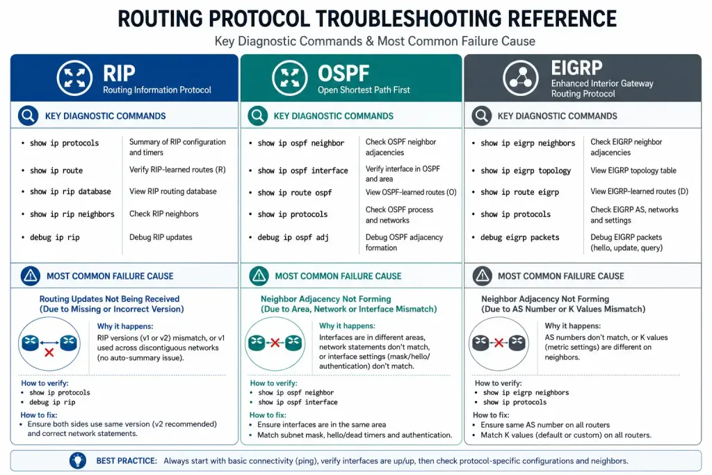
[See Infographic: Troubleshooting Flow by Protocol]
FAQs
What is the difference between static and dynamic routing?
Static routing requires manually configuring every route by hand, with no automatic response to topology changes. Dynamic routing uses protocols like RIP, OSPF, and EIGRP to automatically discover networks and adapt routing tables as the network changes, at the cost of additional protocol overhead and complexity that static routing avoids entirely.
What are the advantages of dynamic routing over static routing?
Dynamic routing scales far better on larger or frequently changing networks, since it doesn’t require manual reconfiguration every time a link fails or a new network is added. This comes with real trade-offs, though — more CPU and bandwidth overhead, and a genuine security surface that a routing protocol introduces, which static routing avoids entirely by not running a protocol at all.
How does Distance Vector routing work, and why is it loop-prone?
Distance-vector protocols like RIP share their entire routing table with directly connected neighbors periodically, trusting that information without independently verifying the actual topology. This “routing by rumor” approach makes them susceptible to routing loops when a neighbor’s information goes stale, which is exactly why loop-prevention mechanisms like split horizon are a core, necessary part of how these protocols function, not an optional add-on.
What is the role of the SPF algorithm in Link-State routing?
The SPF (Dijkstra’s) algorithm calculates the shortest path to every destination using each router’s own complete topological database, built from flooded LSAs describing every link in the area. Because every router in an area runs this calculation independently against the same shared topology information, link-state protocols avoid the stale-information problem that makes distance-vector protocols prone to loops.
Which dynamic routing protocol is best for large networks?
OSPF and EIGRP are generally preferred for larger networks due to better scalability and faster convergence than RIP, whose 15-hop limit and slower convergence make it genuinely unsuitable once a network grows beyond a small size. The specific choice between OSPF and EIGRP often comes down to vendor environment (EIGRP being Cisco-proprietary, historically, versus OSPF’s open standard status) and existing organizational expertise more than a clear technical winner in every scenario.
Is EIGRP really a hybrid protocol?
It’s commonly taught that way, and the label isn’t wrong exactly — EIGRP does include link-state-like features such as maintaining a topology table beyond just the best route. Current Cisco documentation more precisely describes it as an “advanced distance-vector” protocol, since its core DUAL (Diffusing Update Algorithm) mechanism is fundamentally distance-vector in nature, just with substantial enhancements for faster convergence and loop avoidance layered on top.