OSPF (Open Shortest Path First) relies on “cost” as its metric to select the best path in a network. For CCNA and CCNP students, understanding OSPF cost calculation is essential for exam topics covering route selection and path optimization. The default reference bandwidth is 100 Mbps (10^8 bps), and lower costs indicate preferred paths. This metric reflects the relative overhead of sending packets over an interface, naturally prioritizing higher-bandwidth links for faster routing decisions. For how the underlying interface bandwidth value gets configured and verified in the first place, see the dedicated guide on that topic.
The OSPF Cost Formula
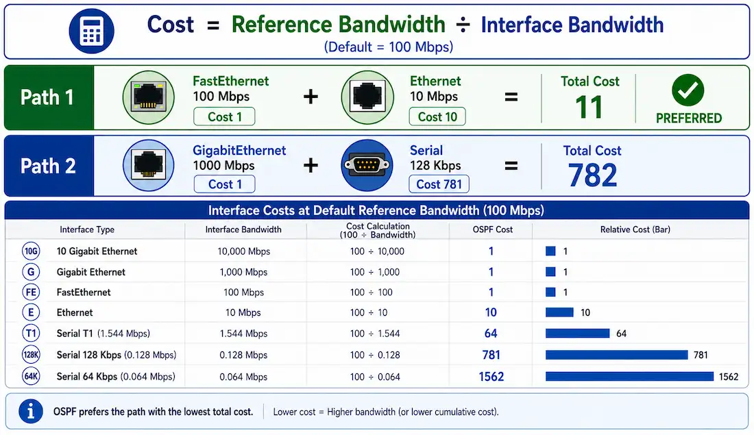
The cost is inversely proportional to bandwidth: higher bandwidth produces a lower cost. Under default settings, a 100 Mbps link has a cost of 1, while a 10 Mbps link has a cost of 10.
Cost = Reference Bandwidth (bps) / Interface Bandwidth (bps)- Default reference bandwidth: 100,000,000 bps (100 Mbps)
- Cisco IOS truncates (floor division) the result to the nearest whole integer
- If the calculated result is less than 1, the cost is set to the hard-coded minimum of 1, since OSPF costs must always be positive integers
Example: For a 100 Mbps interface: 100,000,000 / 100,000,000 = 1. For a 1 Gbps interface: 100,000,000 / 1,000,000,000 = 0.1, which falls below 1 and is therefore set to the minimum cost of 1, not rounded to any other value.
This default reference bandwidth does not differentiate between any links faster than 100 Mbps, since all of them mathematically compute to less than 1 and are floored to the same minimum cost of 1. This leads to suboptimal path selection in modern networks built on Gigabit-plus interfaces, where OSPF cannot tell the difference between a 1 Gbps, 10 Gbps, or 100 Gbps link using the default reference value.
OSPF Cost at Default Reference Bandwidth (100 Mbps)
| Interface Type | Bandwidth (bps) | OSPF Cost |
|---|---|---|
| 10 Gigabit Ethernet | 10,000,000,000 | 1 |
| Gigabit Ethernet | 1,000,000,000 | 1 |
| Fast Ethernet | 100,000,000 | 1 |
| Ethernet | 10,000,000 | 10 |
| Serial (T1, 1.544 Mbps) | 1,544,000 | 64 |
| Serial (128 Kbps) | 128,000 | 781 |
| Serial (64 Kbps) | 64,000 | 1562 |
A note on rounding: every value above is calculated by truncating (flooring) the division result, not by rounding to the nearest whole number. For example, the Serial 128 Kbps calculation is 100,000,000 / 128,000 = 781.25, which truncates down to 781, not up to 782. The only case where OSPF adjusts a value upward is the specific floor-of-zero scenario described above, where any calculated cost below 1 is set to the fixed minimum of 1; this is a hard-coded minimum, not a general “round up” rule, and it is worth being precise about this distinction since it is a commonly tested and commonly misunderstood CCNP-level nuance.
OSPF Accumulates Costs Along the Path
OSPF sums the cost of every outgoing interface along the path from source to destination; incoming interface cost is not used in this calculation, an important and frequently tested distinction.
Example Topology:
Path 1: R1 --FastEth(cost 1)--> R4 --Eth 10Mbps(cost 10)--> R2
Path 2: R1 --GigEth(cost 1)--> R3 --Serial 128Kbps(cost 781)--> R2- Path 1 total cost: 1 + 10 = 11 (preferred, lower total cost)
- Path 2 total cost: 1 + 781 = 782
Even though Path 2 begins with a much faster Gigabit Ethernet link, its second hop is a slow 128 Kbps serial link, making its total accumulated cost far higher than Path 1’s. OSPF selects Path 1 because the total accumulated cost along the entire path is what matters, not the speed of any single link in isolation. Router R1’s routing table for the destination network reached via this path would show an OSPF metric of 11, confirming this calculation. Verify this in a lab with show ip route.
Adjusting the Reference Bandwidth
Because the default 100 Mbps reference bandwidth cannot differentiate between Fast Ethernet and anything faster, the reference bandwidth should be modified to a higher value in any network containing Gigabit-or-faster links, to allow OSPF to make genuinely informed path decisions across the full range of interface speeds present in the network.
Changing the reference bandwidth does not affect the actual physical bandwidth capacity of any link; it only affects the value OSPF uses in its cost metric calculation. Configure it in router configuration mode:
Router(config)# router ospf 1
Router(config-router)# auto-cost reference-bandwidth 1000
The value is specified in Mbps. To adjust for Gigabit Ethernet links, use 1000; for 10 Gigabit Ethernet, use 10000. This configuration must be applied identically on every router in the OSPF domain. A mismatched reference bandwidth between routers causes each router to calculate costs on a different scale, which can result in inconsistent path selection or, in more complex topologies, asymmetric routing where traffic takes a different path in each direction.
To reset the reference bandwidth back to its default value, either explicitly configure it back to 100, or use the more idiomatic reset command:
Router(config-router)# no auto-cost reference-bandwidthOSPF Cost at Reference Bandwidth 1000 Mbps
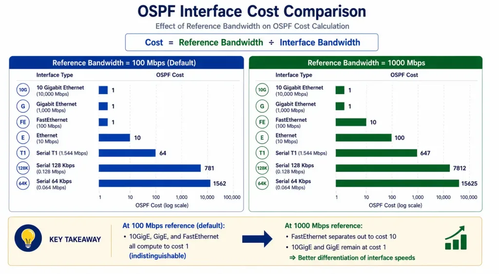
The table below shows the OSPF cost if the reference bandwidth is set to Gigabit Ethernet (1000 Mbps). With this reference value, OSPF can now correctly differentiate between Fast Ethernet and Gigabit Ethernet links, something the default 100 Mbps reference could not do.
| Interface Type | OSPF Cost |
|---|---|
| 10 Gigabit Ethernet (10 Gbps) | 1 |
| Gigabit Ethernet (1 Gbps) | 1 |
| Fast Ethernet (100 Mbps) | 10 |
| Ethernet (10 Mbps) | 100 |
| Serial (1.544 Mbps) | 647 |
| Serial (128 Kbps) | 7812 |
| Serial (64 Kbps) | 15625 |
With a reference bandwidth of 1000 Mbps, a Gigabit Ethernet link (cost 1) is clearly preferred over a Serial 64 Kbps link (cost 15625), and Fast Ethernet (cost 10) is now correctly distinguished from Gigabit Ethernet (cost 1), a distinction the default reference bandwidth could not make since both would compute to the same minimum cost of 1.
For a network containing 10 Gigabit Ethernet links, setting the reference bandwidth to 10000 Mbps would similarly allow OSPF to distinguish Gigabit Ethernet (cost 1000) from 10 Gigabit Ethernet (cost 100), rather than both again defaulting to the same minimum cost.
Manually Overriding Cost on a Specific Interface
In addition to adjusting the domain-wide reference bandwidth, Cisco IOS allows the calculated cost to be manually overridden on an individual interface using the ip ospf cost command, applied directly under interface configuration mode:
Router(config)# interface GigabitEthernet0/1
Router(config-if)# ip ospf cost 50
This sets the OSPF cost for that specific interface to a fixed value of 50, regardless of what the reference-bandwidth-based formula would otherwise calculate. This is useful for fine-tuning traffic engineering on a per-link basis, for example, deliberately making one of two equal-bandwidth links less preferred as a backup path, without needing to change the domain-wide reference bandwidth or the interface’s actual configured bandwidth value.
Verifying OSPF Cost
show ip ospf interface
Router# show ip ospf interface GigabitEthernet0/1
GigabitEthernet0/1 is up, line protocol is up
  Internet Address 10.1.1.1/30, Area 0
  Process ID 1, Router ID 1.1.1.1, Network Type POINT_TO_POINT, Cost: 1
Confirms the calculated (or manually overridden) cost currently applied to a specific interface.
show ip route ospf
Router# show ip route ospf
O    192.168.20.0/24 [110/11] via 10.1.1.2, 00:14:22, FastEthernet0/0
The second number in brackets, 11 in this example, is the accumulated OSPF cost metric to reach that destination network, matching the topology example calculated earlier in this guide.
show ip ospf
Router# show ip ospf
Routing Process "ospf 1" with ID 1.1.1.1
 Reference bandwidth unit is 1000 mbps
Confirms the currently configured domain-wide reference bandwidth value.
Common Pitfalls
- Inconsistent reference bandwidth across routers. Since the reference bandwidth is a locally configured value on each router, forgetting to apply the same value on every router in the OSPF domain causes each router to calculate costs on a different scale, leading to suboptimal or asymmetric routing.
- Forgetting the minimum cost of 1. Any link whose calculated cost falls below 1 is set to the hard minimum of 1, not any other rounded value; this is the only upward adjustment OSPF makes.
- Confusing configured bandwidth with actual physical bandwidth. OSPF cost is calculated from the interface’s configured bandwidth value (visible via
show interfacesand adjustable with thebandwidthcommand — see the interface bandwidth guide for configuration and troubleshooting detail), which does not always match the interface’s true physical line rate, particularly on serial and tunnel interfaces where the configured bandwidth value may need to be set manually to reflect reality.
CCNA Exam Pointers
- OSPF cost formula: Reference Bandwidth (bps) / Interface Bandwidth (bps), truncated (floored), with a hard minimum of 1
- Default reference bandwidth: 100 Mbps; does not differentiate any link faster than Fast Ethernet
auto-cost reference-bandwidth [Mbps]— configured in router configuration mode, must match on every router in the domainno auto-cost reference-bandwidth— resets to the 100 Mbps defaultip ospf cost [value]— manually overrides cost on a specific interface, configured under interface configuration mode- OSPF sums cost along the outgoing interfaces only, from source to destination
show ip route ospf— the number in brackets after the administrative distance is the accumulated OSPF costshow ip ospf interface— shows per-interface cost;show ip ospf— shows the domain’s configured reference bandwidth
Conclusion
OSPF’s cost metric, calculated as reference bandwidth divided by interface bandwidth and floored to a whole number with a minimum of 1, is straightforward in principle but has one significant limitation at its 100 Mbps default: it cannot distinguish between any link faster than Fast Ethernet.
Adjusting the reference bandwidth domain-wide with auto-cost reference-bandwidth, consistently across every router, restores OSPF’s ability to make genuinely informed path decisions in networks built on Gigabit and faster interfaces, and the ip ospf cost command provides a further, more surgical tool for overriding cost on individual links when needed. Understanding that OSPF truncates rather than rounds, and that only the minimum-cost floor of 1 represents an upward adjustment, is a precise, testable detail that separates a solid understanding of OSPF metrics from a superficial one.
FAQs
What is the OSPF cost formula and how does it work?
The OSPF cost formula is Reference Bandwidth divided by Interface Bandwidth, both expressed in bits per second, with the result truncated (floored) to a whole number and a hard-coded minimum value of 1. The default reference bandwidth is 100,000,000 bps (100 Mbps), meaning a 100 Mbps interface computes to a cost of exactly 1, while any interface faster than 100 Mbps computes to a value below 1 and is therefore floored to the same minimum cost of 1, which means OSPF cannot differentiate between a 1 Gbps and a 10 Gbps link without the reference bandwidth being adjusted upward.
Why should you adjust the OSPF reference bandwidth?
The default 100 Mbps reference bandwidth cannot distinguish between Gigabit Ethernet, 10 Gigabit Ethernet, or any faster interface, since all of them compute to the same minimum cost of 1 under that default. Setting the reference bandwidth to 1000 or 10000 Mbps via the auto-cost reference-bandwidth command restores meaningful cost differentiation across the full range of interface speeds present in a modern network. This configuration must be applied identically across every router in the OSPF domain to prevent inconsistent path selection or asymmetric routing between routers calculating costs on different scales.
How does OSPF accumulate costs for route selection?
OSPF sums the cost of every outgoing interface along a path from the source router to the destination network, using only outgoing interface cost, not incoming. In a topology where Path 1 consists of a Fast Ethernet link (cost 1) followed by an Ethernet link (cost 10), the total path cost is 11. If Path 2 instead consists of a Gigabit Ethernet link (cost 1) followed by a slow 128 Kbps serial link (cost 781), its total path cost is 782, making Path 1 the preferred route despite Path 2 starting with a much faster first hop. Verify accumulated cost with show ip route ospf, where it appears as the second number in brackets after the administrative distance.
What are common pitfalls in OSPF cost calculation?
The most common pitfall is an inconsistent reference bandwidth configured across different routers in the same OSPF domain, which causes each router to calculate costs on a different scale and can lead to suboptimal or even asymmetric routing. A second common mistake is misunderstanding the rounding behavior: OSPF truncates (floors) non-integer results rather than rounding to the nearest whole number, with the sole exception being the hard-coded minimum cost of 1 applied to any link whose calculated cost would otherwise fall below 1. A third pitfall is confusing an interface’s actual physical bandwidth with its configured bandwidth value, which OSPF actually uses for the calculation and which does not always match physical reality, particularly on serial and tunnel interfaces.
How do I verify OSPF costs in a Cisco network?
Use show ip ospf interface [interface-id] to see the calculated or manually overridden cost applied to a specific interface. Use show ip route ospf to see the total accumulated cost to each OSPF-learned destination network, shown as the second number in brackets after the administrative distance. Use show ip ospf to confirm the domain’s currently configured reference bandwidth value. For Cisco devices specifically, these three commands together provide a complete picture of both the per-interface and the accumulated end-to-end cost calculations, and are the standard toolkit for diagnosing suboptimal OSPF path selection.