A network engineer stares at a traceroute that defies logic — traffic flows across a 10 Mbps satellite link while a 1 Gbps fiber path sits idle. The root cause isn’t a hardware fault. It’s a misconfigured bandwidth metric. Across every major routing protocol and QoS framework, the bandwidth metric quietly dictates which path packets take, how much traffic a link can reserve, and whether an SLA survives the next congestion spike. For CCNA and CCNP candidates, understanding how bandwidth is measured, advertised, and manipulated separates textbook knowledge from troubleshooting skill.
Where Bandwidth Lives in the Routing Table Decision
Routing protocols do not read physical interface speeds directly. They consult a configured bandwidth value — often set in kilobits per second — that acts as the protocol’s view of link capacity. On a Cisco IOS device, the bandwidth interface command overrides reality:
Router(config)# interface GigabitEthernet0/1
Router(config-if)# bandwidth 10000
This tells EIGRP and OSPF that this link is 10 Mbps, regardless of the actual 1000 Mbps line rate.
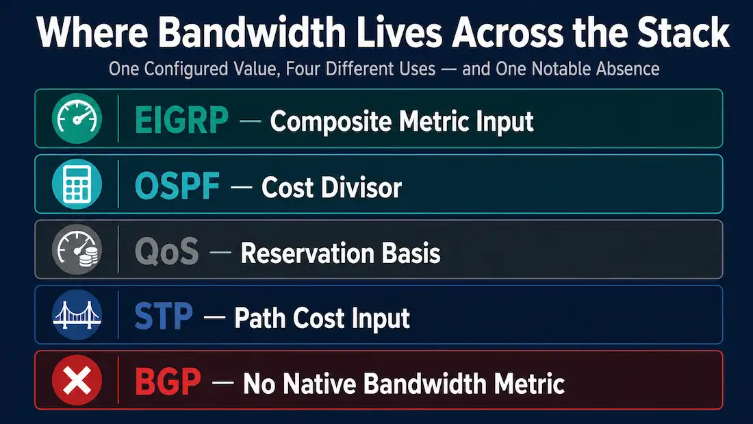
EIGRP and OSPF both use bandwidth, yet their formulas produce radically different outcomes. EIGRP computes a composite metric that, by default, combines bandwidth with delay — load and reliability are also available in the formula but disabled by default. OSPF derives a single cost value based solely on reference bandwidth divided by interface bandwidth. BGP, notably, does not natively carry a bandwidth metric at all — a gap that forces engineers to rely on MED, local preference, or community-tagged policies to steer traffic across AS boundaries.
EIGRP’s Bandwidth-Driven Arithmetic
EIGRP treats bandwidth as a scaled inverse value. In the full composite metric formula, the default (K1=1, K3=1, everything else 0) simplifies to:
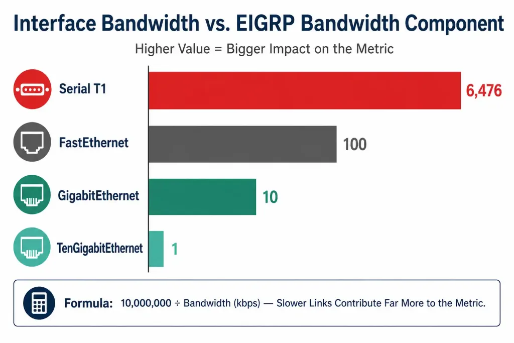
Metric = 256 × (10,000,000 / minimum bandwidth in kbps + cumulative delay in tens of microseconds)Minimum bandwidth is the bottleneck along the entire path — EIGRP takes the slowest link anywhere in the chain, not an average. A single 100 Mbps link in a chain of 10 Gbps links forces the computation to use 100,000 kbps, pulling the metric up sharply regardless of how fast every other segment is.
A note worth being precise about: the composite metric formula uses bandwidth and delay by default, with load and reliability available but disabled. MTU is not part of the formula at all, despite sometimes being grouped alongside the other interface characteristics in casual descriptions — it’s carried in EIGRP Update messages purely as a tiebreaker for specific multi-path scenarios, never as a metric input. Full detail on this distinction, including the exact formula, is covered in EIGRP Composite Metric.
The consequence: an engineer can tune EIGRP path selection by adjusting bandwidth on an interface without touching delay. Changing bandwidth 50000 to bandwidth 5000 inflates the composite metric roughly tenfold, diverting traffic elsewhere. However, delay is often preferred for fine-tuning in practice, because bandwidth changes also influence QoS policies that rely on the same configured value — adjusting bandwidth to steer routing can have side effects on unrelated QoS reservations sharing that same interface. CCNA labs frequently ask candidates to compare outputs of show ip eigrp topology before and after such modifications, while CCIE troubleshooting scenarios require pinpointing a metric mismatch caused by stale bandwidth statements on GRE tunnel interfaces.
| Interface Type | Default Bandwidth (kbps) | EIGRP Bandwidth Contribution (10,000,000/BW) |
|---|---|---|
| Serial T1 | 1,544 | 6,476 |
| FastEthernet | 100,000 | 100 |
| GigabitEthernet | 1,000,000 | 10 |
| TenGigabitEthernet | 10,000,000 | 1 |
OSPF Cost: When Reference Bandwidth Breaks Tie-Breaking
OSPF computes cost as reference bandwidth divided by interface bandwidth. The default reference bandwidth on Cisco devices is 100 Mbps (10⁸ bps), which caps any link faster than 100 Mbps at a cost of 1. This creates a real problem: a 1 Gbps interface and a 10 Gbps interface both appear identical to OSPF, since both compute to the same minimum cost. To restore differentiation, administrators raise the reference bandwidth:
Router(config-router)# auto-cost reference-bandwidth 10000This sets the reference to 10,000 Mbps (10 Gbps), giving OSPF room to differentiate between a 1 Gbps and 10 Gbps link again.
OSPF cost calculation based on reference bandwidth becomes critical in multi-vendor environments. Juniper’s Junos uses a reference bandwidth of 100 Mbps as well, but allows per-VRF cost scaling. When configuring OSPF across VLAN subinterfaces carrying different QoS classes, a mismatch in reference bandwidth between two routers can cause asymmetric routing — traffic out via a low-cost path returns through a high-cost path, breaking stateful firewalls along the way. show ip ospf interface brief instantly shows the computed cost per interface, and the fix usually involves aligning the reference bandwidth across all devices before fine-tuning individual link costs with ip ospf cost.
The BGP Blind Spot: No Native Bandwidth Metric
BGP does not advertise link bandwidth. A BGP next hop represents only reachability, not capacity. This absence becomes acute in SD-WAN fabrics and MPLS L3VPN designs where multiple paths exist with vastly different bandwidth profiles. Modern SD-WAN overlays address this by having the edge device actively probe path characteristics and steer traffic accordingly — latency-sensitive traffic toward low-latency paths, bulk transfer toward high-bandwidth circuits — independent of what BGP itself is advertising.
In traditional BGP, engineers approximate bandwidth awareness by tagging prefixes with communities that map to a local preference or MED value. For example, a prefix learned from a high-bandwidth MPLS PE link might carry a community that a route-map translates into a higher local preference, while a backup path over a lower-bandwidth internet circuit receives a lower one. The absence of an explicit bandwidth metric demands careful documentation, since nothing in BGP itself records or communicates actual link capacity.
QoS and Bandwidth Reservation: Metric Becomes Guarantee
In QoS frameworks, bandwidth transforms from a routing factor into a resource reservation. CBWFQ (Class-Based Weighted Fair Queuing) on Cisco platforms uses the bandwidth and bandwidth remaining percent commands to allocate at least a specified amount of link capacity to a class. A representative LLQ (Low Latency Queuing) configuration for voice on a 2 Mbps serial interface:
policy-map WAN-EDGE
  class VOICE
    priority percent 25
  class CRITICAL-DATA
    bandwidth percent 30
Here, 25% of the configured bandwidth — 500 kbps on a 2 Mbps interface — is policed but prioritized, while 30% is guaranteed for CRITICAL-DATA. If actual throughput dips below the reserved bandwidth due to congestion, packets for CRITICAL-DATA still get dequeued ahead of best-effort traffic.
The catch: the policy-map’s bandwidth percentages refer to the interface’s configured bandwidth statement, not its real clock rate. Setting bandwidth 2048 on a 2 Mbps serial link ensures the math works correctly, but a 1 Gbps Ethernet interface defaults to 1,000,000 kbps — a 30% allocation there would reserve 300 Mbps. An engineer deploying QoS on any interface needs to match the interface bandwidth statement to the actual policed or physical rate, or the reservation logic silently reserves the wrong amount.
Bandwidth vs. Throughput: Why the Metric Lies Without Context
The bandwidth metric represents configured link capacity, not the achievable data rate. Throughput — the actual bits per second crossing the interface — is always lower due to protocol overhead, retransmissions, and congestion. This distinction becomes critical when interpreting SNMP monitoring or flow data: an interface reporting a configured bandwidth of 1 Gbps but showing 150 Mbps of throughput on a monitoring dashboard isn’t necessarily broken; it may be limited by an upstream policer or by TCP windowing across a high-latency path.
When troubleshooting why EIGRP selected a path with lower bandwidth over one with higher bandwidth, checking the delay metric often explains the outcome — delay can swing the composite metric further than bandwidth differences alone in some topologies, since both terms are simply added together in the default formula.
Manipulating Bandwidth Metric in the Lab and Production
CCNP and CCIE candidates encounter bandwidth metric manipulation in routing protocol labs and design tasks regularly. A common scenario: an enterprise runs OSPF between two sites connected by a primary MPLS link and a backup GRE tunnel over the internet.
A version-dependent detail worth getting right: GRE tunnel interfaces do not inherit the bandwidth of the underlying physical path — the default bandwidth assigned to a Tunnel interface has changed across IOS releases. Older IOS versions default a Tunnel interface to 9 kbps; IOS 15.5 and later default to 100 kbps instead. Neither value reflects anything about the tunnel’s actual physical capacity, and both are low enough to badly skew routing decisions if left unconfigured.
With the older 9 kbps default and OSPF’s default 100 Mbps reference bandwidth, the resulting cost is roughly 11,111 (100,000 kbps ÷ 9 kbps) — pushing all traffic toward the MPLS path regardless of the tunnel’s real usability. With the newer 100 kbps default, the cost is a still-very-high 1,000 (100,000 ÷ 100), producing the same practical outcome for a slightly different reason. Either way, the fix is the same:
Router(config)# interface Tunnel0
Router(config-if)# bandwidth 10000
Setting a realistic bandwidth value on the tunnel interface brings its OSPF cost back in line with its actual intended role — whether that’s an active/standby backup or a genuine load-sharing path — and this should be checked and set explicitly on every GRE tunnel rather than relying on either IOS default.
Spanning Tree Also Uses Bandwidth-Derived Cost
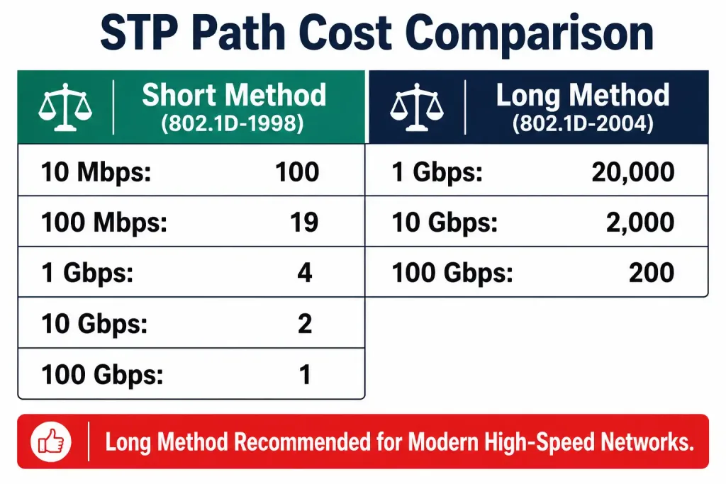
STP (Spanning Tree Protocol) assigns port cost based on link speed too, though the exact values depend on which cost method is active. Under the standard short method (802.1D-1998, still the default on many platforms), the defined costs are: 10 Mbps = 100, 100 Mbps = 19, 1 Gbps = 4, 10 Gbps = 2, and 100 Gbps = 1. Under the long method (802.1D-2004, recommended for modern high-speed networks and enabled via spanning-tree pathcost method long), the values scale differently to preserve differentiation at higher speeds: roughly 1 Gbps = 20,000, 10 Gbps = 2,000, and 100 Gbps = 200.
A misconfigured port bandwidth on a switch can skew STP root port election, diverting traffic through a slower uplink than intended — the same fundamental class of problem as a bandwidth misconfiguration in EIGRP or OSPF, just expressed through STP’s own cost table. VLAN trunks with LACP port-channels combine bandwidth additively; modifying the bandwidth statement on a port-channel interface adjusts routing protocol metrics for that logical bundle as a whole.
Sustainable SLAs and the Bandwidth Metric Feedback Loop
Modern SD-WAN platforms close the loop between bandwidth metric and application performance by actively measuring link latency, jitter, and packet loss, then adjusting path preference dynamically based on the results — rather than relying on a static, once-configured bandwidth number in a routing table. If a link begins degrading, traffic shifts to a healthier path automatically, without requiring manual intervention in the routing configuration itself.
Frequently Asked Questions
Does EIGRP’s composite metric include MTU?
No. Despite occasionally being mentioned alongside bandwidth, delay, load, and reliability, MTU plays no role in the composite metric calculation. It’s carried in EIGRP Update messages purely as a tiebreaker in specific multi-path scenarios.
What’s the correct STP cost for a 100 Gbps link?
Under the standard short method, 100 Gbps carries a cost of 1 — the same as any link fast enough to hit the method’s minimum cost ceiling. Under the long method, which provides more granularity at high speeds, 100 Gbps carries a cost of approximately 200.
Why does a GRE tunnel default to such a low bandwidth value?
Because a tunnel interface has no physical line rate of its own to inherit — it’s a logical construct riding over whatever physical path happens to carry it. Cisco IOS assigns a conservative default (9 kbps on older releases, 100 kbps on IOS 15.5 and later) specifically because there’s no way to automatically know the tunnel’s real usable capacity.
Does changing bandwidth on an interface actually change its physical speed?
No. The bandwidth command only changes the value routing protocols and QoS policies use for their calculations — it has zero effect on the interface’s actual physical clock rate or real throughput capacity.
Why doesn’t BGP use a bandwidth metric like EIGRP or OSPF?
BGP was designed around policy-based path selection between autonomous systems, not raw link-capacity comparison — its attributes (local preference, MED, AS-path length) reflect administrative policy rather than physical link characteristics. Bandwidth awareness in BGP-based designs has to be approximated through community-tagged policy or handled entirely outside BGP, as in modern SD-WAN overlays.
Conclusion
The bandwidth metric is a configurable variable, not a fixed property of a link. Whether it shapes EIGRP composite values, OSPF cost, QoS reservations, STP path selection, or SD-WAN path steering, its power lies in deliberate alignment with real-world capacity and policy intent. Left unconfigured — as with a GRE tunnel’s low default bandwidth, or an OSPF reference bandwidth that hasn’t been raised for modern link speeds — the network will silently route traffic through bottlenecks that a quick glance at the CLI would suggest should never exist.