The best route is the longest match route to the destination IP address. The route lookup process matches the destination IP address with the route available in the routing table and chooses the longest to match route as the forwarding route.
To match the destination IPv4 address of a packet with the routes in the routing table, the minimum number of far-left bits must match the IPv4 address of the packet and the route in the routing table.
The router found the best route in the routing table for the packet using the subnet mask. The data packet never contains the subnet mask in the packet header.
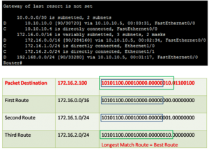
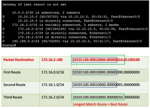
The best route is the longest match or the most significant number of equivalent far-left bits. The figure below illustrates the maximum bits match, which is the best route for the packet.
If the router receives a packet destined for 172.16.2.100, the router has three possible routes for the packet: 172.16.0.0/16, 172.16.1.0/24, and 172.16.2.0/24. Look at the table above in the figure to understand the most prolonged match routing process.
172.16.2.0/24 has the longest match, so the router has selected this route as the best route and forwards the packet to Ethernet 1/1. For any of these routes to be considered a match, there must be at least the number of matching bits indicated by the route’s subnet mask.
Routing Table Terms
The Cisco IP routing table is a hierarchical structure that speeds up the lookup process when locating routes and forwarding packets. Within this structure, the hierarchy includes:
Ultimate route
Level1 route
Level1 parent route
Level2 child routes
Ultimate Route
This route contains either a next-hop IPv4 address or an exit interface. Directly connected, dynamically learned, and local routes are also ultimate routes. The figure below illustrates the ultimate routes.
Level 1 Route
The route that is equal to a subnet mask or less than the classful mask of the network address. The source of the level 1 route can be a directly connected network, a static route, and a dynamic routing protocol. Therefore, a level 1 route is also the ultimate route. The type of level 1 route included:
Network route– A route with a subnet mask equal to the classful network is called a network route.
Default route– This is a static route for the packet whose destination is unknown to the router. The address of the default static route is 0.0.0.0/0.
Supernet route– This route has a network address with a maskless than the classful mask.
Level 1 Parent Route
The Level 1 parent route is a Level 1 network route that is subnetted. A parent route can never be an ultimate route. The figure below illustrates the level 1 parent route highlighted.
The level 1 parent route is the heading for the specific subnets. Each entry displays the classful network address, the number of subnets, and the number of different subnet masks.
Level 2 Child Route
This is a subnet of a classful network address. As illustrated in Figure 1, a level 1 parent route is a level 1 network route that is subnetted. A Level 1 parent route contains Level 2 child routes, as shown in the Figure below.
There are two level 2 child routes for level 1 parent route 10.0.0.0 and three level 2 child routes for level 1 parent route 172.16.0.0. The source of a level 2 route can be a directly connected network, a static route, or a dynamically learned route. Level 2 child routes are also ultimate routes.
Route Lookup Process
When a router receives a packet on an interface, the router examines the packet’s header, identifies the destination IPv4 address, and proceeds through the router lookup process.
Step-1
The router examines level 1 routes, network routes, and supernet routes for the best match with the destination address of the IP packet.
If the best match is a level 1, ultimate, or supernet route, the packet is forwarded to the destination using the best match route.
If the best match is a level 1 parent route, continue to the next step.
Step-2
The router examines level 2 child routes of the level 1 parent route for the best match.
If a match with a level 2 child route is found, the router forwards the packet to the destination using this route.
Continue to the next step if no match is found with any level 2 child routes.
Step-3
The router starts looking up the best match in level 1 supernet routes in the routing table, including the default route.
If there is now a minor match with a level 1 supernet or default route, the router uses that route to forward the packet.
The router drops the packet if a match to the destination is not found with any route in the routing table.
The routers are typically responsible for directing traffic across multiple networks. Each router maintains a list of known networks and directions calling routing table. The router performs a routing table entries lookup to find the proper interface that leads to the destination address. Each entry in a routing table is called a “route entry: or “route”.
The route identifies the destination network to which traffic can be forwarded. The destination network, in the form of an IP address and netmask, can be an IP network, subnetwork, supernet, or host. Routing table entries can originate from the following sources:
Directly connected networks
Dynamic routing protocols, such as EIGRP, OSPF, and RIP
Routes imported from other routers or virtual routers
Statically configured routes
Directly Connected Entries
When the router interface is configured with an IP address and the interface state is up and up, the directly connected route is automatically added to the router’s routing table.
Connected routes always precede static or dynamically discovered routes because they have the administrative distance value of 0 (the lowest possible value). The directly connected routes contain the following information.
Route source is the entry from where the route has been learned. C and L are two route source codes for directly connected routes. C identifies a directly connected network automatically created when an interface is activated and configured with an IP address. L identifies the local route created whenever an interface is configured with an IP address and activated. The L entry did not appear in routing table entries before IOS resale 15.
Destination network– This is the address of the destination network that also shows the connectivity.
The outgoing interface shows the exit interface for packet forwarding to the destination network.
Remote Route Source
A router stores information about both directly connected and remote routes. As with directly connected networks, the route source identifies how the route learned. Common codes for remote networks include:
S– This code Identifies an administrator’s static route to reach a specific network.
D– This code Identifies the dynamically learned route using the EIGRP routing protocol.
O– This code Identifies the dynamically learned route using the OSPF routing protocol.
R– This code Identifies the route learned dynamically from another router using the RIP routing protocol.
Remote Network Routing Table Entries
The figure below displays an IPv4 routing table entry for the route to remote network 192.168.0.0. We can identify the following information from this entry:
Route source– discussed earlier in this lesson.
Destination network– discussed earlier in this lesson.
Administrative distance– Identifies the trustworthiness of the route.
Metric– This is the value assigned to reach the remote network. Lower values indicate preferred routes.
Next hop– Identifies the IPv4 address of the next router.
Route timestamp– Identifies from when the route was last heard.
Outgoing interface– This is the outgoing interface towards the destination.
Only two routing protocols use link-state: Open Shortest Path First (OSPF) and Intermediate System to Intermediate System (IS-IS). Open Shortest Path First (OSPF) and Intermediate System to Intermediate System (IS-IS) share many similarities and differences. Both routing protocols provide the necessary routing functionality.
Open Shortest Path First (OSPF)
The Open Shortest Path First (OSPF) protocol is the most popular protocol that uses link-state. The Internet Engineering Task Force (IETF) designed OSPF in 1987. Currently, the OSPF has two working versions. OSPFv2 for IPv4 networks, as explained in RFC 2328, is an open standard. The second version is OSPFv3 for IPv6 networks, as stated in RFC 2740. The OSPFv3 also supports IPv4 addresses. Open Shortest Path First (OSPF) is an open standard that will run on most routers. Open Shortest Path First (OSPF) uses the Dijkstra algorithm to provide a loop-free topology. It provides fast convergence with triggered and incremental updates via Link State Advertisements (LSAs). It is also a classless protocol and allows for a hierarchical design with VLSM and route summarization.
Intermediate System to Intermediate System (IS-IS)
Intermediate System to Intermediate System (IS-IS) is an open standard routing protocol designed by the International for Standardization (ISO) and described in ISO 10589. It was initially designed for the Open System Interconnection (OSI) protocol suite and not for the TCP/IP protocol suite. Later, Integrated IS-IS, or Dual IS-IS, started providing support for IP networks. Though IS-IS is known as the routing protocol for Internet Service Providers(ISPs) and carriers, more enterprise networks are beginning to use IS-IS. The ISPs and carriers use IS-IS because of its scalability and strength. It is much easier than OSPF to build a large network. IS-IS carries a payload of reachability data, but for the most part, it doesn’t care what’s in the payload.
Link-state routing protocols have several advantages and disadvantages compared to distance vector routing protocols. This article will discuss these advantages and disadvantages.
Advantages of link-state
Fast Network Convergence—Fast network convergence is the main advantage of the link state routing protocol. On receiving an LSP, link state routing protocols immediately flood the LSP out of all interfaces without any changes except for the interface from which the LSP was received.
Topological Map—Link state routing creates the network topology using a topological map or SPF tree. Using the SPF tree, each router can determine the shortest path to each network separately.
Hierarchical Design—Link state routing protocols use multiple areas and create a hierarchical design for the network areas. The multiple areas allow better route summarization.
Event-driven Updates– After the initial flooding of LSPs, the LSPs are sent only when there is a change in the topology and contain only the information regarding that change. The LSP contains only the information about the affected link. The link state never sends periodic updates.
Disadvantages of Link State
The Link-state also has some disadvantages compared to distance vector routing protocols:
Memory Requirements—The link state routing protocol creates and maintains a database and SPF tree, which require more memory than a distance vector protocol.
Processing Requirements—Link state routing protocols require more CPU processing because the SPF algorithm requires more CPU time than distance-vector algorithms, like Bellman-Ford. After all, link-state protocols build a complete map of the topology.
Bandwidth Requirements–The link state routing protocol floods the link-state packet duringinitial startup and at events like network breakdown and network topology changes, affecting the network’s available bandwidth. If the network is not stable, it also creates issues with the bandwidth.
Link-state routing protocols are also known as shortest-path first protocols. They maintain a complete picture of all the routers running a link-state routing protocol in the complete network. All routers running a link-state routing protocol originate information about themselves and their directly connected routers, links, and the state of those links as multicast messages.
The link-state router tries to maintain complete network topology by updating itself whenever a change occurs. Link-state routing protocols are based on the Shortest Path First (SPF) algorithm to find the best path to a destination. The shortest Path First (SPF) algorithm is also known as the Dijkstra algorithm. The OSPF is an example of a Link-State Routing Protocol.
Link State Process
Following is the process of the link-state routing protocol. The process is the same for both OSPF for IPv4 and OSPF for IPv6.
Link and Link-State
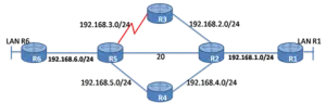
Link and Link-state is the first step in the routing process. Each router learns about its links and directly connected networks. When a router interface is configured with an IP address and subnet mask and also in the state of no shutdown, it becomes part of that network. Refer to the topology in the Figure below. R3 has just been added to the network, and the IP addresses on the router interface are not configured yet; only the physical connectivity has been done. So, the router is not part of Link-State.
The network administrator now configured the IP addresses of the router interfaces connected to R2 and R5 and changed the state of interfaces from shutdown to no shutdown. As they become active, R3 learns about its own directly connected networks. Without any routing protocols, these directly connected networks are now entries in the routing table.
The router’s interfaces must be accurately configured with IP addresses and subnet masks, and the link must be in the state of no shutdown before the link-state routing protocol can learn about a link. Also, like distance vector protocols, the interface must be included in one of the network router configuration statements before participating in the link-state routing process.
Link-state routers have direct information from all their neighbor routers. Each router originates information about itself, its directly connected links, and the state of those links. This information is passed around the network from router to router, and each router makes a copy of it without changing it. So, every router gets identical information about the internetwork, and each router will independently calculate its best paths.
In the reference topology, the R3 link to its directly connected networks are:
FastEthernet 0/0 – 192.168.2.0/24
FastEthernet 0/1 – 192.168.3.0/24
The link-state information includes the following information:
The interface’s IPv4 address and subnet mask
The type of network, such as Ethernet or Serial link
The cost of that link
Any neighbor routers on that link
The link state of R3 is the following:
Link1
Network: 192.168.2.0/24
IP address: 192.168.2.1
Type of network: Ethernet
Cost of that link: 10
Neighbours: None
Link2
Network: 192.168.3.0/24
IP address: 192.168.3.1
Type of network: Serial
Cost of that link: 64
Neighbours: None
Hello Protocol
The second step in the link-state routing process is the responsibility of meeting with neighbors on directly connected networks. Routers with the link-state routing protocol use a Hello protocol for establishing and maintaining router-neighbor relationships. A neighbor is any other router enabled with the same link-state routing protocol. The link-state routing protocol uses Hello packets for neighbour discovery and also for recovery.
The protocol continues exchanging Hello packets between two adjacent neighbors and serves as a keep-alive function to monitor the neighbor’s state. Suppose any router stops receiving Hello packets from a particular neighbor. This neighbor is considered unreachable, so the link-state protocol clears this router from adjacency.
Now refer to Figure 1 above, R1 sends Hello packets to it’s all interfaces when the administrator configures it, to discover the link-state neighbours .R2, and R3 respond to the Hello packet with their own Hello packets as these routers have configured with the same link-state routing protocol as shown in figure 2. The FastEthernet 0/0 interface has no neighbors. So R1 did not receive any hello on this interface; therefore, it does not continue with the link-state routing process steps for the FastEthernet 0/0 link.
OSPF Hello Packet
After the primary exchange of Hello Packet, the routers add each other to their Neighbor Tables. The Neighbour table is the list of connected OSFP-enabled routers. Hello, packets are not recorded in the OSPF database, but if the hello packet has not been received from a particular neighbor for 40 seconds. The link-state routing protocol marked this particular neighbor as down. For example, OSPF will not take any notice if a link goes down for 20 seconds and again comes back to up status.
If a link goes down from a minute to half an hour, OSPF floods an LSA when it goes down and another LSA when it is up again. If a link is down for over half an hour, LSAs originated by remote routers begin to age out. When the link returns, all these LSAs will be flooded again. If a link is down for over an hour, any LSAs originated by remote routers will have aged out and been flushed. The link will be like a new OSPF route when it comes back up.
Building the Link State Packet (LSP)
The third step in the link-state routing process is building the link-state packet (LSP) containing the state of each directly connected link. It carries the information a network router generates in a link-state routing protocol that lists the router’s neighbors. It is a datagram determining the names of routers, including the cost or distance to any neighboring routers and linked local networks. It can also choose a new neighbor In case of link failure. The LSP also determines what the new neighbor is if a link fails and the cost of changing a link if required.
LSPs are queued for transmission and must time out at about the same time. The network is used to distribute the LSP but cannot use the routing database. When a router has established adjacencies to other routers, it can build its LSP containing the link-state information about its links. Now refer to the figure below. The LSP from R1 should contain the information like the following:
R1; FastEthernet network 192.168.0.0/24; Cost 1
R1 -> R2; Serial point-to-point network; 192.168.1.0/24; Cost 1
R1 -> R3; Serial point-to-point network; 192.168.3.0/24; Cost 1
Flooding LSP
After building the LSP, each router floods the LSP to all neighbours in the link-state routing process. This is the fourth step in the link-state routing process. The neighbor routers receive the LSP and save it in the database. All routers in the same routing area flood the link-state information to each other.
When a router receives the LSP from any of its interfaces, then the receiving router immediately sends that LSP out to all interfaces except the receiving interface. This process continues from router to router in the same area until all routers receive the LSP. When flooding LSP is completed then the link-state routing protocol calculates the SPF algorithm, thus the link-state routing convergence speed is very high.
The routers do not send LSPs periodically like the hello packet. They are only sent during the initial startup of the routing protocol on the router. After that, the LSPs are needed to flood when network changes occur in the topology. They are also required when a network breakdown occurs or after the network comes back.
The LSPs also included information, such as sequence numbers and aging information, to help manage the flooding LSP process. Each router uses this information to determine if it has received the LSP from another router or has new and updated information than the LSP already contained in the link-state database. This process allows a router to keep only the most current information in its link-state database. Suppose we discuss the topology in the previous lesson, building the Link State Packet. The R1 will flood the LSP packet to all its interfaces containing the following data.
R1; FastEthernet network 192.168.0.0/24; Cost 1
R1 -> R2; Serial point-to-point network; 192.168.1.0/24; Cost 1
R1 -> R3; Serial point-to-point network; 192.168.3.0/24; Cost 1
Building the SPF Tree
The routers in the same area use the link-state database and SPF algorithm to build the SPF tree. For example, in the figure below, R1 builds the SPF tree using the link-state information from all other routers. The SPF algorithm reads the router’s LSP to recognize networks and the link’s costs.
In the first step, R1 identifies its directly connected networks and their costs. After identifying the directly connected network, R1 begins identifying unknown networks from R2 and R3. Then, the SPF algorithm calculates the shortest paths to reach each network.
The SPF algorithm then calculates the shortest paths to reach each network. Each router in the area builds its own SPF tree separately from all other routers. To ensure accurate routing, the link-state databases used to construct those trees must be identical on all routers.
Building the Link-State Database
Link-state database building is the last step in the link-state routing process. Each router in the link-state uses the database to build a complete map of the topology and computes the best path to each destination network. All routers receive LSPs from every other link-state router in the same routing area. the
These LSPs are stored in the link-state database. Each router maintains a separate link-state database for every area to which it belongs, in case more than one area is configured in the network. The link-state database is also referred to as the topological database, and routers belonging to the same area have the same topological database for the area.
The databases for each area always process separately and calculate the link-state shortest path separately for each area and the topological database. The shortest path is flooded throughout the respected area only. The area database build of router links advertisements, network links advertisements, and summary link advertisements included external routes in all non-stub area databases.
Summary of Link-State Process
Every router in an OSPF area will complete the following link-state process to exchange a state of convergence:
Each router learns about its own directly connected networks and Links by detecting the interfaces in the upstate.
All routers are responsible for “saying hello” to their neighbors on directly connected networks.
Each router builds a Link-State Packet (LSP) containing the state of each directly connected link—the LSP contains neighbor, neighbor ID, link type, and link bandwidth.
Each router floods the LSP to all neighbors. Those neighbors store all LSPs received in a database. They then flood the LSPs to their neighbors until all area routers have received them LSPs. Each router stores a copy of each LSP received from its neighbors in a local database.
Each router floods the LSP to all neighbors, storing all LSPs received in a database.
All routers use the database to build a complete topology map and calculate the best path to each destination network using Dijkstra’s Algorithm.
Important Term of Link-State Protocol
Topological database – It is a set of information collected from LSAs.
SPF algorithm– The shortest path first (SPF) algorithm is a calculate the SPF tree on the bases of information in the database.
Routing tables – A list of the known paths and interfaces.
LSA – A link-state advertisement (LSA); is a small packet of routing information that is sent among routers. It is a basic communication way of the OSPF routing protocol for the Internet Protocol (IP). It communicates the router’s local routing topology to all other local routers in the same OSPF area.
LSP – It is a packet containing information generated by a network router in a link-state routing protocol that lists the router’s neighbours. It is a special datagram determining the names of routers including the cost or distance to any neighbouring routers and linked local networks. It can also determine the new neighbour In case of link failure.