Interarea route summarization must be manually configured on an ABR — OSPF has no auto-summarization feature. Once configured, the ABR condenses multiple specific routes from one area into a single Type 3 Summary LSA before forwarding it into the backbone. This guide focuses specifically on the part most guides skip: how to actually calculate the summary address and mask by hand, using binary matching, before ever touching the configuration command — and, just as importantly, how to check afterward exactly what a calculated summary does and doesn’t cover.
This is a companion to OSPF Route Summarization, which covers both inter-area and external summarization more broadly. This article goes deeper into the arithmetic behind the inter-area case specifically.
What Triggers a Summary Route
Two behaviors worth knowing before configuring area range:
A summary route only generates if at least one component subnet actually exists. If none of the area’s current subnets fall within the specified summary range, OSPF won’t generate an empty summary LSA — there has to be at least one real, active subnet for the summary to have anything to represent. This matters in practice: a network engineer pre-configuring a summary range in anticipation of subnets that haven’t been deployed yet will see no summary route appear at all until at least one matching subnet actually comes online.
The summary’s advertised cost is the lowest cost among all the routes it summarizes, not the highest and not an average. This is the default Cisco IOS behavior for area range summaries, and it means a summary route’s metric can understate the actual cost to reach some of the more distant subnets it covers — worth keeping in mind when troubleshooting a path that seems to route somewhere with the “wrong” apparent cost, since the discrepancy is expected behavior rather than a sign of a misconfiguration.
The ABR performing the summarization can only summarize routes from areas it’s actually connected to — it can’t reach into an area it has no interface in and summarize routes there.
Calculating a Summary Address in Three Steps
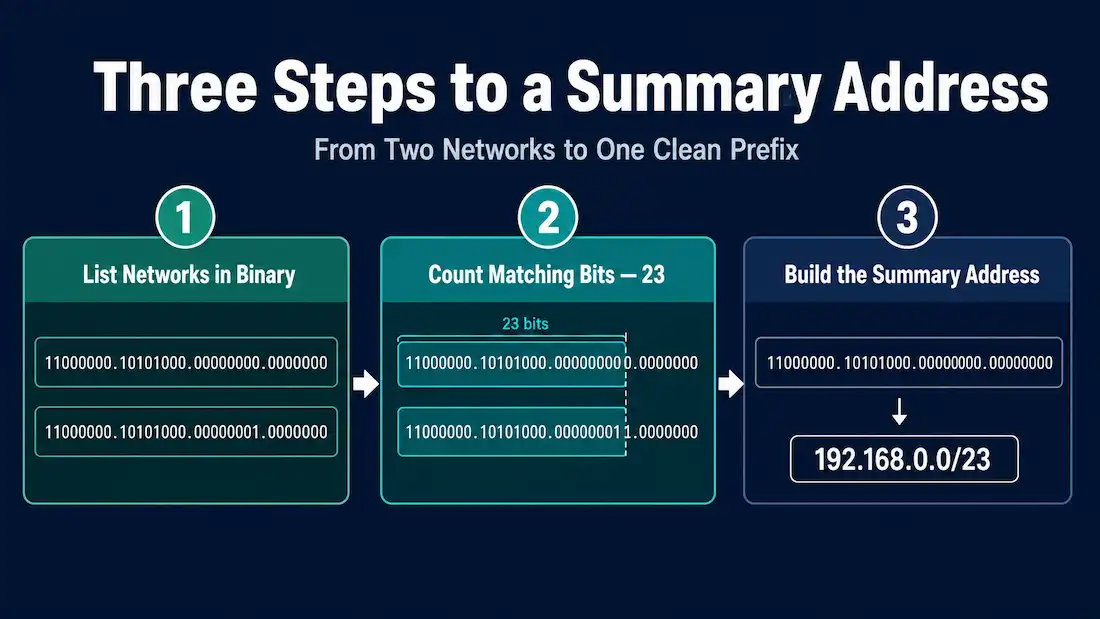
Summarizing adjacent subnetworks into a single address and mask comes down to three steps, worked here with a concrete example: summarizing 192.168.0.0/24 and 192.168.1.0/24, two networks both originating in Area 10.
Step 1: List Every Network in Binary
192.168.0.0/24  →  11000000.10101000.00000000.00000000
192.168.1.0/24  →  11000000.10101000.00000001.00000000
Step 2: Count the Matching Bits, Left to Right
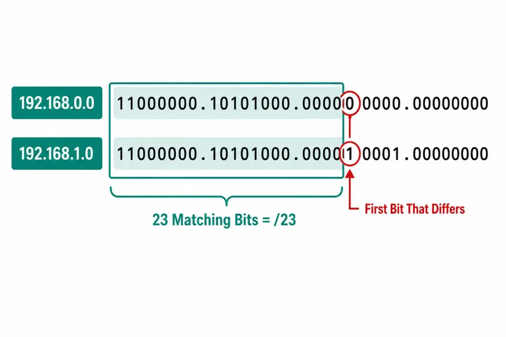
Comparing the two addresses bit by bit from the left: the first two full octets (11000000.10101000) match completely — that’s 16 bits. Moving into the third octet, 00000000 versus 00000001 — the first 7 bits match (0000000), and the bits diverge at the 8th bit of that octet (0 versus 1). That gives 16 + 7 = 23 matching bits total.
Twenty-three matching bits means a /23 prefix — a subnet mask of 255.255.254.0.
Step 3: Build the Summary Address
Take the matching bits exactly as they are, and set every remaining bit to zero:
11000000.10101000.00000000.00000000Converted back to decimal, that’s 192.168.0.0. Combined with the /23 mask calculated in Step 2, the resulting summary address is 192.168.0.0/23 — a single route that correctly covers both 192.168.0.0/24 and 192.168.1.0/24 without including any address space beyond those two networks.
Configuring the Calculated Summary
With the address and mask worked out, configuring it on the ABR is a single command. In this topology, R2 is the ABR connecting Area 10 to Area 0 (the backbone), and R2 — not any internal router within Area 10 — is where the summarization command belongs, since only an ABR can perform inter-area summarization:
R2(config)# router ospf 10
R2(config-router)# area 10 range 192.168.0.0 255.255.254.0
R2(config-router)# do write
This tells R2 to summarize any routes it holds for Area 10 that fall within 192.168.0.0/23, advertising the single summarized address into the backbone rather than the individual /24 routes.
OSPFv3 Syntax
The equivalent OSPFv3 command follows the same logic, differing only in using IPv6 prefix notation instead of an address/mask pair:
Router(config-rtr)# area <area-id> range <prefix>/<prefix-length>Verifying the Result
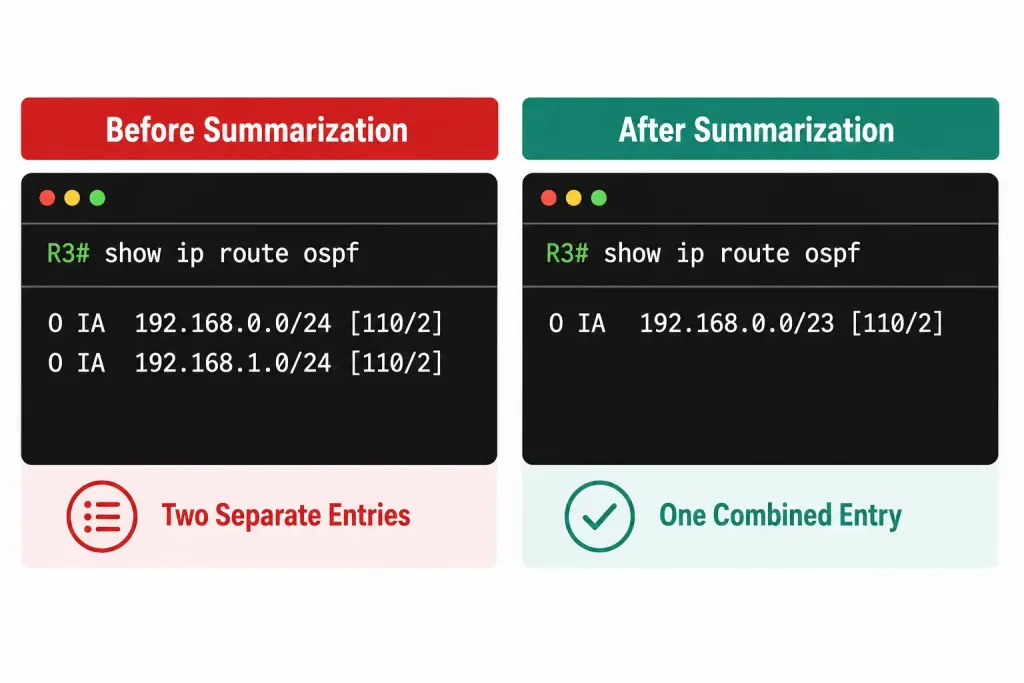
Before configuring the summary, a router elsewhere in the OSPF domain — one that never had the specific 192.168.0.0/24 and 192.168.1.0/24 networks configured locally — would show both as separate inter-area entries:
R3# show ip route ospf
O IA  192.168.0.0/24 [110/2] via 10.10.10.1
O IA  192.168.1.0/24 [110/2] via 10.10.10.1
After the summarization command takes effect on R2, that same router’s routing table collapses both entries into one:
R3# show ip route ospf
O IA  192.168.0.0/23 [110/2] via 10.10.10.1
In this small example, summarization only reduced the routing table by a single entry — going from two routes to one. The real benefit scales with the size of the area being summarized: an area with twenty subnets that all fit cleanly under one summary mask collapses down to that same single entry, which is where interarea summarization earns its value in a larger network, and why the technique is worth mastering even when a two-network toy example doesn’t look especially impressive on its own.
Practicing the Calculation with a Harder Example
The two-network example above works cleanly because the two subnets differ by only a single bit. Real networks are rarely quite that tidy. Consider summarizing three networks instead: 192.168.4.0/24, 192.168.5.0/24, and 192.168.6.0/24 — a case chosen deliberately because it doesn’t divide as neatly as the first example, and illustrates a subtlety worth understanding before relying on this technique in a real design.
In binary, the third octet of each is 00000100, 00000101, and 00000110. Comparing all three together, the matching bits from the left are 000001 — six bits — before the values diverge (the remaining two bits vary across the three networks: 00, 01, 10). Combined with the 16 matching bits from the first two octets, that’s 16 + 6 = 22 matching bits, giving a /22 summary.
Applying that mask, the summary address becomes 192.168.4.0/22. It’s worth checking this result carefully: a /22 covers four consecutive /24 networks — in this case 192.168.4.0/24 through 192.168.7.0/24. The three networks being summarized (.4, .5, .6) are covered, but so is 192.168.7.0/24, which was never part of the original set. If no such network exists in the area, this is completely fine — the summary just doesn’t have anything using that particular /24, which doesn’t cause any problem on its own. But it’s a useful habit to double-check exactly which addresses a calculated summary actually spans, since it’s easy to assume a summary covers only the specific networks you started with.
Working Backward: Checking What a Given Summary Actually Covers
The reverse skill — starting from a summary address and mask, and working out exactly which specific networks it covers — comes up just as often in practice, particularly when troubleshooting an unexpected route or verifying someone else’s existing configuration.
Given area 20 range 172.16.8.0 255.255.252.0, the /22 mask means the block size in the third octet is 4. Starting from 172.16.8.0, the covered range runs through 172.16.11.255 — meaning any /24 from 172.16.8.0 through 172.16.11.0 falls inside this summary, while 172.16.7.0/24 and 172.16.12.0/24 do not, even though they might look adjacent at a glance. Getting this boundary right matters when diagnosing why a particular subnet either is or isn’t being correctly summarized — a subnet just one number outside the calculated range won’t be included, full stop.
Common Mistakes
Assuming the summary only covers the exact input networks. As the three-network example shows, a summary mask defined by matching bits can (and often does) cover more address space than the specific set of networks that motivated the calculation. Always verify what the resulting mask actually spans before assuming a summary is exactly as narrow as intended.
Configuring the summarization command on the wrong router. Only an ABR (or an ASBR, for external routes) can summarize. A common mix-up is writing the configuration against an internal router by mistake — the command will simply have no meaningful effect there, since that router isn’t in a position to translate Type 1/2 LSAs into a Type 3 summary in the first place, and internal routers don’t sit at an area boundary where this translation happens.
Forgetting that a summary route needs at least one real subnet to represent. If every subnet that would have fallen within a planned summary range gets removed or renumbered out of that range, the summary LSA disappears too — this is expected behavior, not a fault, but it can be confusing if you’re specifically expecting to see a summary route that no longer has anything to summarize.
Frequently Asked Questions
How do I know how many bits will match between two networks without writing out the full binary?
For networks that differ only in their last octet, a quick shortcut: two consecutive numbers (like .0 and .1) typically differ starting somewhere in the low-order bits, and the number of matching bits corresponds to how large a power-of-two block both numbers fall within together. Writing out the binary directly, at least while learning, remains the most reliable way to get this right and to catch cases like the four-network span example above.
Does the ABR need routes from both areas to summarize, or just the source area?
Just the source area specified in the area <area-id> range command — that’s the area whose routes are being condensed. The summary is then injected toward the other areas the ABR is connected to, most commonly the backbone.
What happens to the summary’s cost if the component routes have very different costs?
The summary advertises the lowest cost among all the routes it covers, by default. This means paths to some of the summarized subnets may show a lower advertised cost from outside the area than their true internal cost, which is a normal, expected side effect of summarization rather than a misconfiguration.
Can I summarize non-contiguous networks together?
Only if their binary representations happen to share enough matching leading bits to express a mask that covers them — which for genuinely scattered, non-adjacent networks, often means the resulting summary mask ends up covering far more address space than intended. Planning subnets in contiguous blocks from the start makes clean summarization possible; trying to force a summary onto poorly planned, scattered addressing usually doesn’t work well.
How do I check which specific networks a summary I didn’t configure myself actually covers?
Work backward from the mask: figure out the block size the mask implies (for example, a /22 has a block size of 4 in whichever octet the summary boundary falls in), then list out the full range starting from the summary’s base address. This tells you definitively which specific subnets fall inside the summary and which fall just outside it, which is often the fastest way to explain an unexpected routing result during troubleshooting.
Conclusion
Calculating an OSPF summary address comes down to three mechanical steps: write the networks in binary, count how many leading bits match, and build the summary address from those matching bits with zeros everywhere else. The math itself is straightforward once practiced, but the real skill is checking what a calculated summary actually covers — since matching bits alone can pull in more address space than the specific networks that motivated the calculation, especially once more than two networks are involved. Being equally comfortable working the calculation forward (from networks to a summary) and backward (from a summary to the networks it covers) is what turns this from a memorized procedure into something genuinely useful for day-to-day troubleshooting.