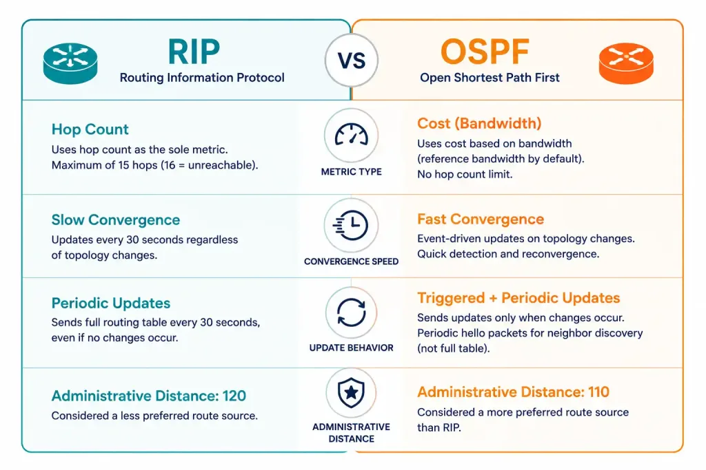
Open Shortest Path First is a link-state routing protocol built to replace RIP, the distance-vector protocol that worked reasonably well in early, small networks but never scaled. RIP’s hop-count metric ignores bandwidth entirely and its full periodic table broadcasts don’t hold up as networks grow — problems OSPF was specifically designed to solve.
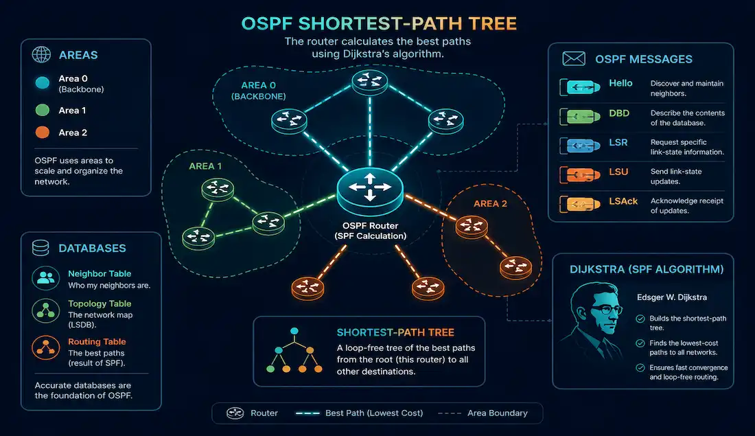
Open Shortest Path First offers real advantages over RIP: it scales to much larger networks, converges far faster after a topology change, and is a classless routing protocol built around the concept of areas for hierarchical scaling. OSPF uses Dijkstra’s SPF algorithm, created by computer scientist Edsger Wybe Dijkstra, to calculate the best path to every destination from a complete map of the network topology.
The Development of Open Shortest Path First
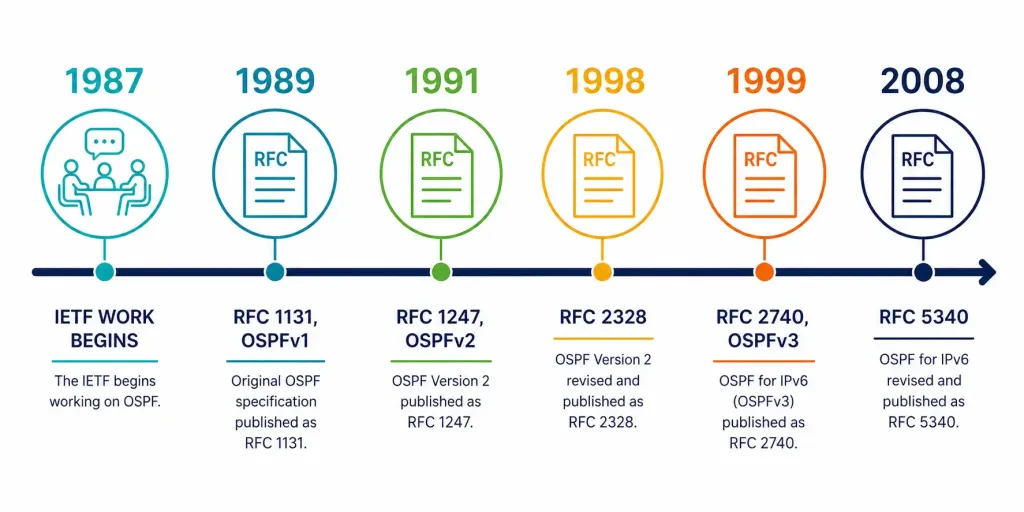
The IETF began initial work on OSPF in 1987, at a time when the internet itself wasn’t yet public — it existed only as an academic and research network funded by the United States government. OSPF version 1 was published in 1989 as RFC 1131, intended to run on routers and UNIX workstations, and its implementation later became widespread through a UNIX process known as GATED. OSPFv1 was experimental and was never actually deployed in production.
In 1991, John Moy introduced OSPF version 2 in RFC 1247, a significant improvement that made the protocol classless and added support for VLSM and CIDR. Around the same time, the IETF selected OSPF as its recommended interior gateway protocol (IGP). RFC 2328, published in 1998, updated OSPFv2 and remains the current base specification for OSPFv2 to this day.
OSPF version 3 — OSPF for IPv6 — arrived in RFC 2740 in 1999, authored by Rob Coltun, Dennis Ferguson, and John Moy. It was updated again in 2008 in RFC 5340, which remains the current specification for OSPFv3.
Key Features of OSPF
- Classless — OSPF is classless by design, giving it full support for VLSM and CIDR.
- Fast convergence — Changes propagate quickly through the network rather than waiting for the next periodic update cycle.
- Efficient — OSPF has no periodic full-table updates; it triggers routing updates only in response to actual topology events, using the SPF algorithm to select the best path each time.
- Scalable — OSPF works well in both small and large networks, and grouping routers into areas supports a genuinely hierarchical design as a network grows.
- Secure — OSPF supports MD5 authentication. Once MD5 is enabled, a router only accepts routing updates from peers presenting the same pre-shared key, protecting against unauthorized or forged updates.
- Trustworthy by design — OSPF carries a default administrative distance of 110, which places it ahead of RIP (120) but behind EIGRP’s internal routes (90) when multiple sources offer routes to the same destination.
Components of OSPF
It divides a network into smaller areas, which keeps individual routing tables smaller and topology databases more manageable — a direct benefit of not every router needing to know every detail about the entire network. Every OSPF network includes a backbone Area 0, which links every other area together, plus a set of hardware components, databases, messages, and the algorithm that ties it all together.
Hardware Components
Area Border Routers (ABRs) sit at the boundary between one or more OSPF areas, forming the link between the backbone and each attached area.
AS Boundary Routers (ASBRs) exchange routing information with networks outside the OSPF autonomous system entirely, advertising externally learned routes into the OSPF domain. An ASBR can simultaneously function as an ABR, a backbone router, or an internal router, depending on where it physically sits in the topology — but a router inside a stub area specifically cannot act as an ASBR, since stub areas are defined by their inability to carry Type 5 LSAs, which is exactly what an ASBR would need to advertise external routes.
OSPF Areas
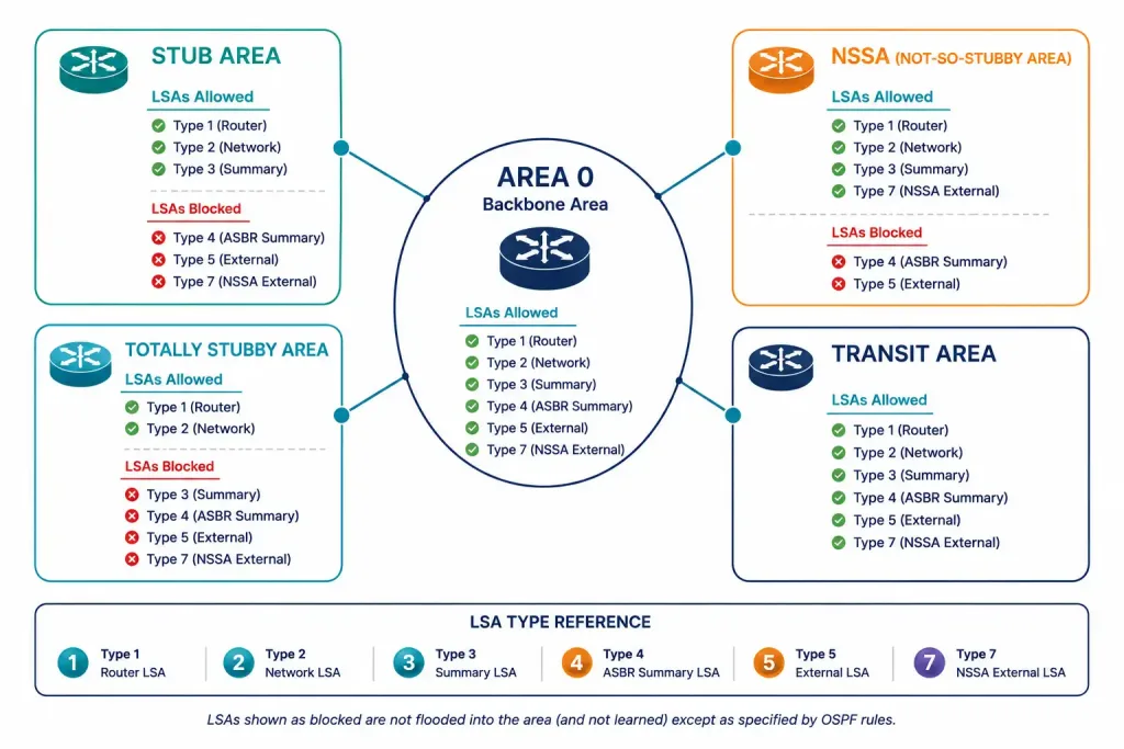
Splitting a single autonomous system into smaller areas reduces the number of LSAs flooded across the network and shrinks the topology database each individual router has to maintain.
- Backbone area — Area 0.0.0.0, which every other area connects to and through which inter-area routing information is distributed. The backbone is itself an area, so ordinary area rules and terminology apply to it as well.
- Stub areas — areas shielded from external (AS-level) route advertisements, while still receiving routing information about other areas within the same OSPF domain. Routers inside a stub area rely on a default route, originated by that area’s ABR, to reach anything outside the OSPF domain — the ABR must have a default metric configured before it can advertise that default route.
- Not-So-Stubby Areas (NSSA) — combine most of a stub area’s benefits with the ability to import external route information from within the NSSA itself, which then gets leaked into other areas. External routes originating from other areas, however, still don’t enter an NSSA.
- Totally stubby areas — filter OSPF database information by LSA type specifically: the ABR prevents Type 3, 4, and 5 LSAs from being flooded into the area at all, replacing all of them with a single default route.
- Transit areas — areas through which a virtual link can be configured. A transit area needs full routing information and, by definition, cannot itself be a stub area.
OSPF Databases
It maintains three distinct databases, each serving a different purpose in building and maintaining the router’s view of the network:
- Adjacency database — maintains the neighbor table, tracking which routers this router has established bidirectional communication with. Being neighbors doesn’t automatically mean two routers are adjacent — on a multi-access network, two routers only become fully adjacent if at least one of them is the Designated Router (DR) or Backup Designated Router (BDR) for that segment. View this database with
show ip ospf neighbor. - Link-state database (LSDB) — builds the topology table for every area a router belongs to, made up of router LSAs, network LSAs, and summary LSAs, and also maintains a list of every router in the network. View it with
show ip ospf database. - Forwarding database — the router’s actual routing table, listing how and where to send a packet to reach each known destination. View it with
show ip route.
DR and BDR Election on Multi-Access Networks
The DR/BDR concept mentioned above deserves a bit more explanation, since it’s central to how OSPF scales on shared segments like Ethernet. On a multi-access network with several OSPF routers, having every router form a full adjacency with every other router would create an unnecessary flood of redundant LSA exchanges — with N routers on a segment, that’s roughly N²/2 adjacencies to maintain.
Instead, OSPF elects one router as the Designated Router and a second as the Backup Designated Router; every other router on that segment forms a full adjacency only with the DR and BDR, dramatically reducing the number of adjacencies and the volume of LSA flooding needed to keep everyone synchronized. This election is based on OSPF priority first, with the router ID as a tiebreaker.
Routing Protocol Messages
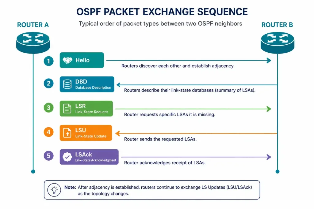
OSPF routers exchange five types of packets to discover neighbors and build accurate routing information:
- Hello packet — discovers neighboring routers and maintains existing adjacencies.
- Database Description (DBD) packet — summarizes the contents of a router’s link-state database during the initial synchronization process.
- Link-State Request (LSR) packet — requests specific, more detailed LSAs a router is missing.
- Link-State Update (LSU) packet — floods the actual LSAs in response to a request, or when a topology change occurs.
- Link-State Acknowledgment (LSAck) packet — confirms receipt of an LSU, ensuring reliable delivery across the flooding process.
The Algorithm
OSPF is a link-state protocol, meaning it uses local CPU resources to process the neighbor and topology tables through Dijkstra’s SPF algorithm — a cumulative, cost-based calculation for reaching every destination in the topology. The algorithm builds a shortest-path tree, calculating the lowest-cost path to each node from the local router’s perspective. OSPF then installs the resulting best routes into the forwarding database, which becomes the actual routing table used to forward traffic.
OSPF Neighbor States
Forming an adjacency isn’t instantaneous — routers progress through a defined sequence of states as they discover each other and synchronize their databases. Seeing where a stuck adjacency stalls in this sequence is one of the most useful OSPF troubleshooting skills.
- Down — no Hello packets have been received from this neighbor yet.
- Init — a Hello has been received, but it doesn’t yet list the local router’s own ID, so two-way communication isn’t confirmed.
- 2-Way — both routers have seen each other in their Hello packets, confirming bidirectional communication. On multi-access networks, DR/BDR election happens at this stage, and routers that won’t become fully adjacent (neither DR, BDR, nor DROther peers of each other) stay at 2-Way rather than progressing further.
- ExStart — the two routers negotiate which one will lead the database synchronization process, based on router priority and ID.
- Exchange — routers exchange Database Description packets, summarizing what each has in its link-state database.
- Loading — routers send Link-State Request packets for any detailed LSAs they’re missing, and receive them via Link-State Update packets.
- Full — the two routers have fully synchronized link-state databases and are considered completely adjacent.
show ip ospf neighbor displays each neighbor’s current state directly, making it the first command to check when an adjacency isn’t forming as expected — a neighbor stuck at 2-Way on a point-to-point link, for instance, points toward a very different problem than one stuck at ExStart.
Frequently Asked Questions
What is Open Shortest Path First?
It is a link-state routing protocol developed by the IETF, starting in 1987, specifically to replace RIP’s limitations in larger networks. It uses Dijkstra’s SPF algorithm to calculate the genuinely shortest path to every destination based on a complete topology map, rather than relying on hop count or secondhand neighbor information the way RIP does. OSPF is classless, supports VLSM and CIDR, and scales through a hierarchical area-based design that keeps individual routers’ topology databases manageable even in large networks.
What are the key features of OSPF?
It is classless, supports fast, event-triggered convergence rather than periodic full-table updates, and scales well through its area-based hierarchy. It supports MD5 authentication to secure routing updates against unauthorized peers, and it carries a default administrative distance of 110, placing it between EIGRP’s internal routes (90) and RIP (120) in terms of route preference when multiple protocols offer paths to the same destination.
What are OSPF areas, and what are the different types?
it divides a network into areas to reduce the number of LSAs flooded and the size of the topology database each router has to maintain. The backbone area (Area 0) connects every other area together; stub areas block external route advertisements while still relaying information from other areas within the domain; Not-So-Stubby Areas combine stub-area benefits with the ability to import their own external routes; totally stubby areas go further and filter out inter-area summary LSAs as well, replacing everything with a single default route; and transit areas support virtual links and therefore can’t themselves be configured as stub areas.
What databases does OSPF maintain, and how do I view them?
OSPF maintains three databases: the adjacency database, which tracks neighbor relationships and is viewed with show ip ospf neighbor; the link-state database (LSDB), which holds the full topology map for each area a router belongs to and is viewed with show ip ospf database; and the forwarding database, which is simply the router’s actual routing table, viewed with the familiar show ip route. Each database serves a distinct role in the process of discovering neighbors, building a shared topology view, and ultimately selecting and installing the best paths.
How does OSPF use Dijkstra’s algorithm to calculate routes?
OSPF runs Dijkstra’s SPF algorithm locally on each router’s CPU, using the complete topology information stored in the link-state database to calculate the cumulative lowest-cost path to every other router and network in the area. The algorithm builds a shortest-path tree rooted at the local router, and the resulting best paths are installed into the forwarding database, which becomes the router’s actual routing table. Because every router in an area runs this same calculation against the same shared topology data, the result is consistent, loop-free routing throughout the entire OSPF domain.