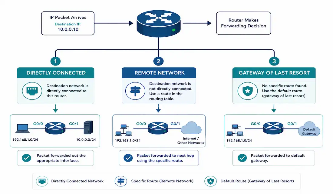
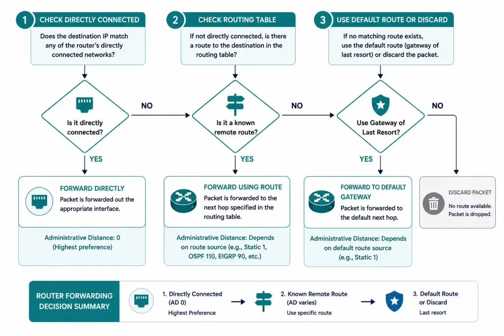
Every time a router receives a packet, it runs through the same basic decision sequence: is the destination directly connected, is it a remote network reachable through a known route, or is there no known route at all? Understanding this sequence — and exactly how a router picks between multiple valid paths when more than one exists — is foundational CCNA and CCNP material, and it’s the logic behind nearly every routing troubleshooting session you’ll ever run.
This guide walks through all three destination categories, how the Gateway of Last Resort fits in, how RIP, OSPF, and EIGRP each calculate their own “best path” differently, and a complete worked example tying it all together.
Directly Connected Networks
A directly connected network is any subnet matching one of the router’s own configured interfaces. When you assign an IP address to an interface, the router automatically creates a directly connected route in its routing table — no additional configuration required. These routes carry an administrative distance of 0, making them always preferred over any other route source to the same destination.
Verify directly connected routes:
Router# show ip route connected
C        192.168.1.0/24 is directly connected, GigabitEthernet0/0
C        10.0.0.0/24 is directly connected, GigabitEthernet0/1
The C prefix indicates a connected route, with the interface showing exactly where that network is physically attached.

Remote Networks
If a packet’s destination doesn’t match any directly connected subnet, it’s a remote network — reachable only through a next-hop router, learned via static configuration or a dynamic routing protocol.
View remote routes:
Router# show ip route
R    172.16.0.0/16 [120/1] via 192.168.1.2, 00:00:05, GigabitEthernet0/0
The R prefix indicates a route learned via RIP. The bracketed values [120/1] show the administrative distance (120, RIP’s default) and the metric (1 hop) respectively, followed by the next-hop address, how long ago the route was learned, and the exit interface.
No Known Route: The Gateway of Last Resort
If a packet’s destination doesn’t match a directly connected network, a remote route, or any other entry in the routing table at all, the router falls back to its default route — commonly called the Gateway of Last Resort. If no default route is configured, the packet is simply discarded.
Configure a default route:
Router(config)# ip route 0.0.0.0 0.0.0.0 192.168.1.2Verify it:
Router# show ip route
S*   0.0.0.0/0 [1/0] via 192.168.1.2
The S* prefix specifically marks this as the default route — note the administrative distance of 1 (standard for a static route) and metric of 0. Without this entry present, debug ip routing can help confirm packets are actually being discarded due to a missing default route, rather than some other failure.
Best Path Selection When Multiple Routes Exist
When a router has genuinely multiple paths to the same destination — through different exit interfaces — it needs to select the best one using a protocol-specific metric. Lower metric wins, and administrative distance is only relevant between different protocols; when comparing paths within the same protocol, the metric alone decides.
How Each Protocol Calculates Its Metric
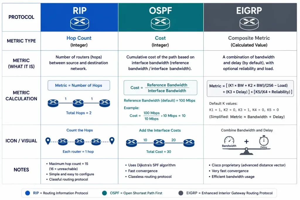
| Protocol | Metric | Calculation |
|---|---|---|
| RIP | Hop count | Number of routers to the destination; fewer hops preferred |
| OSPF | Cost | 10⁸ ÷ bandwidth in bps (with default reference bandwidth) |
| EIGRP | Composite metric | Combines bandwidth, delay, load, and reliability |
RIP is the simplest: a 2-hop path beats a 3-hop path, full stop, regardless of the actual bandwidth or quality of either path — a real limitation that’s part of why RIP has fallen out of favor for anything beyond small, simple networks. A 2-hop path over a pair of slow, congested links will always be chosen over a 3-hop path across fast, uncongested ones, purely because RIP has no way to factor bandwidth or congestion into its decision at all.
OSPF cost, with Cisco’s default reference bandwidth of 100 Mbps, gives a 100 Mbps link a cost of exactly 1 (10⁸ ÷ 10⁸ = 1). This is worth understanding precisely, because it has a well-known modern gotcha: any link at or above 100 Mbps — Gigabit Ethernet, 10 Gigabit Ethernet — also computes to a cost floor of 1 with the default reference bandwidth, since OSPF cost doesn’t go below 1. On a network with faster-than-Fast-Ethernet links, this means OSPF can’t actually distinguish between a Gigabit and a 10 Gigabit path by cost alone unless auto-cost reference-bandwidth is manually raised to reflect current link speeds:
Router(config-router)# auto-cost reference-bandwidth 10000Setting this to 10000 (representing 10 Gbps) recalibrates the cost formula so modern high-speed links are actually differentiated from each other, rather than all clustering at cost 1.
EIGRP combines bandwidth, delay, load, and reliability into one composite metric, which generally makes it more precise than RIP’s blunt hop count, at the cost of more complexity to calculate by hand.
A Complete Worked Example
Consider Router1 with two possible paths to reach 172.16.0.0/16:
- Path A: via GigabitEthernet0/1, a 1 Gbps link, OSPF cost = 1 (with default reference bandwidth)
- Path B: via GigabitEthernet0/2, a 100 Mbps link, OSPF cost = 1 (also, due to the reference bandwidth limitation above)
With default settings, OSPF sees both paths as equally costed and installs both for equal-cost load balancing — even though Path A genuinely offers ten times the bandwidth. After adjusting auto-cost reference-bandwidth to 10000, the same two paths recalculate to cost 1 (Path A) and cost 10 (Path B) respectively, and OSPF now correctly prefers Path A exclusively.
This example is exactly why the reference bandwidth gotcha matters in practice, not just as a trivia fact: a network administrator who never adjusts the default can end up load balancing across links of meaningfully different capacity, believing OSPF is making an informed choice when it’s actually working from stale assumptions about what counts as “fast.” This is worth checking proactively on any network with links faster than 100 Mbps, rather than waiting for a performance complaint to trigger the investigation — a quick review of auto-cost reference-bandwidth against your actual link speeds takes far less time than diagnosing an unexplained performance issue after the fact.
When Administrative Distance Ties: A Common Point of Confusion
It’s worth addressing a scenario that trips people up: what happens if two different routing protocols both offer a route to the exact same destination with genuinely identical administrative distance? In practice, this is rare by design — Cisco deliberately assigns different default AD values to each protocol specifically to avoid this ambiguity (EIGRP internal at 90, OSPF at 110, RIP at 120, and so on), so a true tie only happens if an administrator has manually changed a protocol’s AD to match another’s, which is unusual and generally discouraged unless there’s a very specific reason for it.
If a genuine AD tie did occur, the router’s behavior in that edge case depends on the specific IOS version and platform, which is part of why relying on default AD values — rather than manually tuning them into collision — is the standard, safer practice. This is a good example of why administrative distance and metric solve two different problems: AD exists specifically to create a clear, unambiguous hierarchy between different protocols, while metric handles the finer-grained comparison within a single protocol once AD has already narrowed things down to one source.
Route Summarization’s Effect on Path Selection
It’s also worth understanding how summarized routes interact with this decision process, since summarization is common on any network of meaningful size. When a router summarizes multiple specific subnets into one larger advertised route, downstream routers see only the summary — they lose visibility into which specific path within that summary might actually be shorter or faster for a given destination.
This is a deliberate trade-off: summarization reduces routing table size and improves convergence time, but it can occasionally mean traffic takes a technically suboptimal path to reach a specific subnet buried within a larger summarized block, simply because the more specific routing information never made it that far. Understanding this trade-off matters for anyone designing route summarization policy, not just for troubleshooting an existing network.
Troubleshooting Path Selection Issues
A route you expect isn’t showing up in the routing table: confirm the routing protocol is actually running and has formed neighbor relationships (for OSPF/EIGRP) or is actively exchanging updates (for RIP).
Router# show ip route
Router# show ip protocols
Traffic is taking a worse path than expected: check the actual metric values being used, particularly for OSPF where the reference bandwidth issue above is a common, easy-to-miss cause.
Router# show ip ospf interface GigabitEthernet0/1 | include CostPackets to an unknown destination aren’t being discarded as expected, or are being routed unexpectedly: verify whether a default route actually exists and where it points.
Router# show ip route 0.0.0.0Suspected routing table inconsistency during troubleshooting: debug ip routing shows routing table changes in real time, though it should be used cautiously on a production router given the console output volume it can generate under an actively changing topology.
Router# debug ip routingAlways disable debugging when you’re done investigating:
Router# undebug allFAQs
What is the role of administrative distance in router path selection?
Administrative distance determines which route source is preferred when multiple protocols offer a route to the same destination — a directly connected route (AD 0) is always preferred over a RIP-learned route (AD 120), for instance. Lower AD values always win between different protocols, but AD isn’t used to compare two routes learned from the same protocol; that comparison relies on the protocol’s own metric instead.
How does a router handle packets destined for a remote network?
The router consults its routing table for a matching entry and forwards the packet to the associated next-hop address or exit interface. If multiple valid paths exist to that same remote network, the router’s routing protocol metric decides which one (or ones, in the case of equal-cost load balancing) actually gets used.
What happens if a router has no route for a packet’s destination?
The router checks for a Gateway of Last Resort — a configured default route. If one exists, the packet is forwarded there; if not, the packet is discarded entirely, which can be confirmed by checking show ip route for the presence or absence of a S* default route entry.
How does OSPF determine the best path, and what’s the reference bandwidth gotcha?
OSPF calculates cost as 10⁸ divided by a link’s bandwidth in bps, with the path having the lowest cumulative cost winning. With Cisco’s default 100 Mbps reference bandwidth, any link at or above that speed computes to the same cost floor of 1, meaning OSPF can’t distinguish a Gigabit link from a 10 Gigabit link without manually raising auto-cost reference-bandwidth to reflect current network speeds.
Why is EIGRP considered more precise than RIP for path selection?
EIGRP’s composite metric factors in bandwidth, delay, load, and reliability together, rather than relying purely on hop count the way RIP does. This lets EIGRP make meaningfully better-informed decisions on networks where hop count alone doesn’t reflect which path is actually fastest or most reliable.
How can I troubleshoot a router that seems to be choosing the wrong path?
Start with show ip route to see which routes and metrics are actually installed, then check protocol-specific details — like OSPF interface cost with show ip ospf interface — to understand why a particular metric came out the way it did. debug ip routing can show real-time routing table changes, but it’s worth using cautiously and disabling promptly afterward on a production device given the volume of output it can generate.